This document outlines the operation and functionality of the Signal Hound Spike™ spectrum analyzer software. Spike™ is compatible with Signal Hound's line of spectrum analyzers and tracking generators which include:
- PCR Series - PCR4200
- SM series – SM200A / SM200B / SM200C / SM435B / SM435C
- SP series – SP145A / SP145B
- BB series – BB60A / BB60C / BB60D
- SA series – SA44 / SA44B / SA124A / SA124B
- TG series – TG44 / TG124
A TG series device can only be interfaced when a compatible spectrum analyzer is connected in the Spike software.
This document will guide users through the setup and operation of the software. Users can use this document to learn what types of measurements the software is capable of, how to perform these measurements, and how to configure the software.
Software Updates
The latest version of the Spike software is always available at www.signalhound.com/Spike. The software will also alert a user when a newer version of the software is available. This alert will appear in the status bar as well as on the Help > About Spike dialog. The software will provide a link to where the latest version can be downloaded.
Preparation
System Requirements
Supported Operating Systems
- Windows 11/10 64-bit
- Ubuntu 18.04 and newer, 64-bit
- PCR, SM, SP, and BB devices only
Processor requirements:
- x86-64 Intel/AMD processors
- Recommended: Intel 4+ core processors (i5/i7/i9)
- Higher speed devices and higher demand processing can require more powerful CPUs.
Our software is highly optimized for Intel CPUs. We recommend them exclusively. Xeon processors are not recommended.
RAM requirements: The software will on average require less than 1GB of memory. Certain configurations for the BB and SM products can consume several GB of memory.
- Recommended: 8 GB
- Minimum: 4 GB
Peripheral Requirements:
- SM435B, SM200B/A, BB60D/C/A - USB 3.0 type-A port
- SP145 - USB 3.0 type-C port with 10W power delivery, or USB 3.0 using an external power supply.
- SM435C, SM200C - 10GbE network connectivity through NIC via SFP+ connectors or through Thunderbolt 3 to SFP+ adapter. See the network setup guide for more information.
- SA44/SA124 - USB 2.0
Graphics drivers: OpenGL 3.0 support required.
We do not recommend running Signal Hound products in a virtual machine (e.g., Parallels, VMWare).
Software Installation
Software Installation (Windows)
The most current version of the software can be found on our website at www.SignalHound.com/Spike.
Once you have downloaded the software, run Spike Installer(x64).msi or Spike Installer(x86).msi and follow the on-screen instructions. You must have administrative privileges to install the software. The installer will install the USB 3.0 drivers for the SM, SP, and BB series devices. The SA and TG series USB 2.0 drivers must be downloaded and installed separately from www.signalhound.com/Spike.
It is recommended to install the application in the default directory.
Note: It is becoming more common for customers to need to enable the High Performance power plan in Control Panel > Power Options. If you are using a low power or ultra-portable PC or laptop, consider this step to ensure optimal performance. See Power Management Settings for more information.
Software Installation (Linux)
Download the latest Linux Spike application at www.signalhound.com/spike. Follow the installation instructions found in the README file included in the download.
Driver Installation
Driver Installation (Windows)
The drivers for the SA series devices must be downloaded and installed separately. Visit www.signalhound.com/Spike to download the USB drivers. The installer must be run as administrator.
The drivers for the USB 3.0 devices are placed in the application folder during installation. The \drivers\x86\ folder is for 32-bit systems and the \drivers\x64\ folder is for 64-bit systems. The drivers should install automatically during setup.
If the drivers did not install correctly, you can manually install them:
- Navigate to the application folder and locate Drivers64bit.exe (or Drivers32bit.exe for 32-bit systems).
- Right-click and select Run as administrator. The console output will confirm whether the installation was successful.
If that does not work, verify that the driver files are in their respective folders. You can also right-click the .inf file in the driver folder and select Install.
If drivers still do not install properly, contact Signal Hound.
Driver Installation (Linux)
Signal Hound USB devices use the libusb driver on Linux. Please follow all installation instructions found in the README file in the Linux application download.
Connecting Your Signal Hound
With the software and device drivers installed, you are ready to connect your device. Connect the supplied USB cable to the PC first, then to the device. If your device includes a Y-cable, ensure both USB ends are connected to the PC before connecting the device.
Once connected, verify the device has been properly recognized by the computer by checking the device manager under the Universal Serial Bus Controllers tab.
Once connected, run Spike. The first time a device is run on a new PC, it may require additional initialization time.
If your device uses a 10GbE network connection, refer to the separate network configuration manual for additional instructions.
Running the Software for the First Time
Once the software and drivers have been installed and the device is connected to the PC, launch the software via the desktop shortcut or the Spike.exe file found in the installation directory. The default installation directory on Windows is:
C:\Program Files\Signal Hound\Spike
If a USB device is connected or an Ethernet device's network address has been saved when the software is launched, the software will attempt to open the device immediately.
If no device is connected and no Ethernet device's address has been saved, the software will notify you. If multiple devices are found, a selection dialog will appear allowing you to choose which device to connect. Select Cancel to enter idle mode. In idle mode, a device can be opened using File > Connect Device.
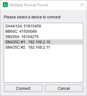
Multiple Devices Found Dialog
If your device is connected and Spike still reports no devices found, see the Troubleshooting section.
Getting Started
This section describes the user interface (UI) in detail and how it can be used to control your Signal Hound spectrum analyzer.
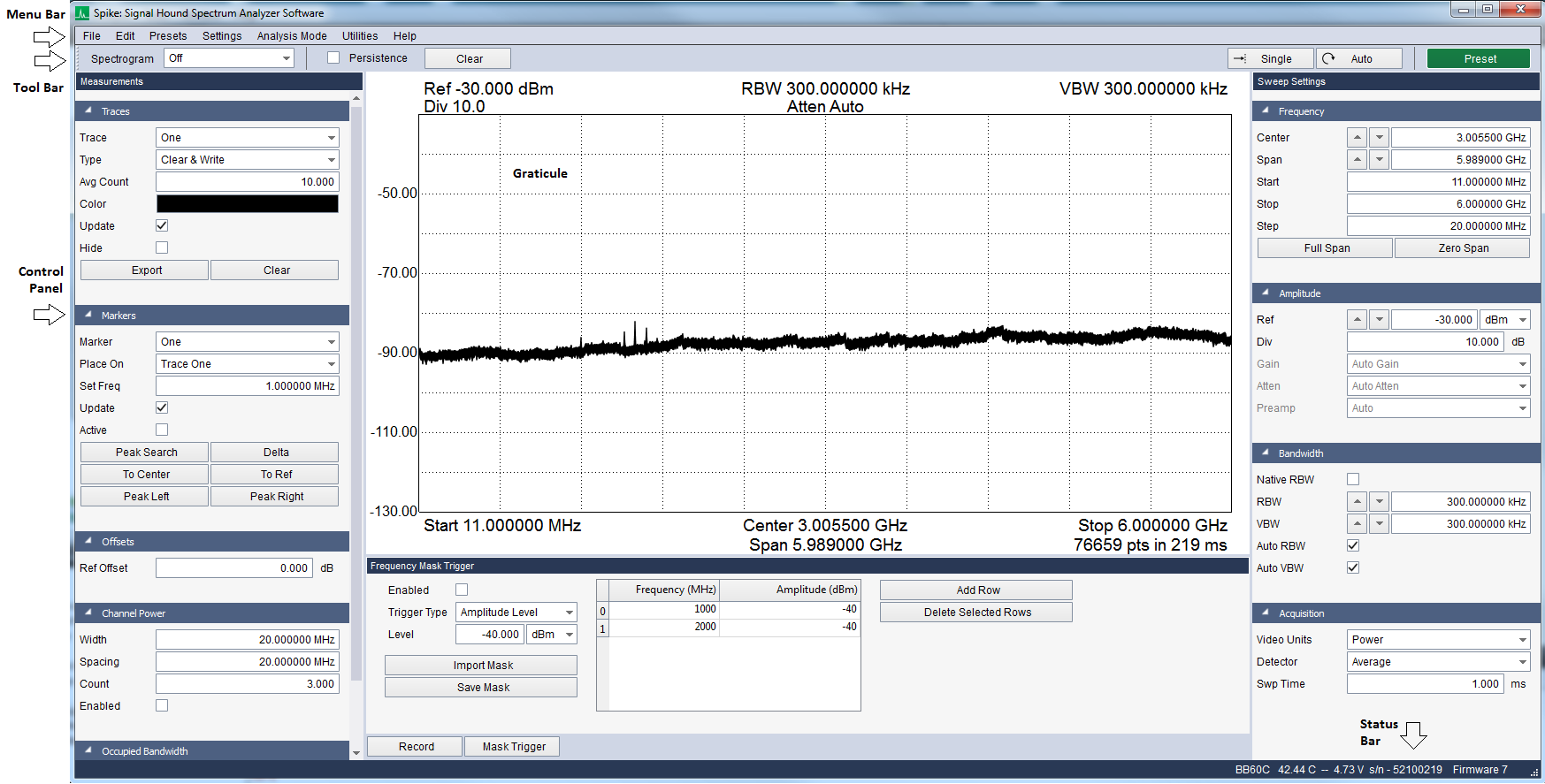
Spike User Interface after Launch
The Menu Bar
File Menu
- Load User Preset – Load a user-selected preset. See Presets Menu for more information.
- Save User Preset – Save a user-selected preset. See Presets Menu for more information.
- Print – Print the current view. Whether control panels are included alongside the graticule is configured in Preferences > Screenshot Settings > Include Control Panels in Image.
- Save as Image – Save the current view as a PNG, JPG, or BMP image.
- Quick Save Image – Capture the current view as a PNG image without specifying a file name or save location. Files are named in increasing order prefixed with SpikeImage. The save directory is the last directory used to save an image file, defaulting to MyDocuments/SignalHound if no image has been saved previously.
- Manage Correction Data – Open a dialog to view and clear correction data files for your Signal Hound devices. See Correction Data for more information.
- Connect Device – If no device is connected, this will attempt to discover all Signal Hound devices connected via USB and list them by serial number. Saved network devices are listed by name. A single device can be selected from this list.
- Manage Ethernet Devices – Open a dialog to add, edit, and remove name and addressing information for Signal Hound networked devices. See Network Devices for more information.
- Disconnect Device – Disconnects the currently connected device. Useful for cycling device power or swapping devices without closing the software.
- Exit – Disconnect the device and close the software.
Edit Menu
- Restore Default Layout – The software will restore its original layout the next time the application is launched.
- Set Title – Enable or disable a custom title. The title appears above the graticule and is included in screen captures and session recordings.
- Clear Title – Remove the current title.
- Hide Control Panels – Temporarily hides all visible control panels. Useful for presentations or small resolution displays.
- Show Control Panels – Shows any control panels that were previously hidden. Control panels are automatically shown when the mode changes or a preset is loaded.
- Theme – Select a color theme for the application. This sets every color in the Colors section of the Preferences dialog.
- Preferences – Opens a configuration dialog for further software configuration.
Presets Menu
Presets are an easy way to store and load measurement configurations. Each preset stores the full software configuration, making it easy to switch between setups and pick back up where you left off. Preset files use the .ini extension.
The Spike software supports three methods for storing and loading presets:
- Via File menu — save and load explicit preset files by selecting .ini files directly.
- Via Presets menu — up to 9 presets are available for quick use, loadable with keyboard shortcuts.
- Power on preset — saved from the Presets menu, this preset loads automatically when a device is connected.
Presets can only be loaded by the same device type that was used when the preset was saved.
Quick presets are stored at:
C:\Users\YourUserName\AppData\Roaming\SignalHound\
AppData\ is a hidden folder by default on Windows systems.
Each quick preset is stored in its own folder labeled Preset [1-9]. The main file has the .ini extension and is named Preset [1-9].ini. The power on preset is named PowerOnPreset.ini. To use a preset on a different computer, copy the preset folder to the correct path on the new machine.
The power on preset can be deleted from the Presets menu or manually deleted from the filesystem.
Settings Menu
Analysis Mode Menu
This menu option allows you to switch between the main measurement modes in Spike.
Utilities Menu
- Error Info - Displays a list of any errors generated during the operation of the software.
- Path Loss Tables – See Path Loss, Limit Line, and Antenna Factor Format for more information.
- Limit Lines – See Managing Limit Lines for more information.
- Audio Player – See Audio Player for more information.
- Measuring Receiver – See Using the Measuring Receiver Utility for more information.
- Frequency Difference Meter – See Frequency Difference Meter for more information.
- Timebase Adjustment – See Adjusting Your Timebase for more information.
- Tracking Generator Controls – If a SA or BB series spectrum analyzer is the active device and a Signal Hound tracking generator is connected to the PC, this utility adds a control panel for manually controlling the tracking generator output. The tracking generator will only respond if scalar network analysis mode is not active.
- SA124 IF Output – Opens a dialog to control the IF downconverter for SA124 spectrum analyzers. While the SA124 IF downconverter is active, the device cannot perform other tasks.
- SM435 IF Output – Control the SM435 as an IF downconverter. The SM435 device must have the IF output option. It can function as a 24–43.5 GHz to 1.5 GHz downconverter with 800 MHz of bandwidth. No other measurements can be performed while the device is in this mode.
- Self-Test – Opens a dialog for manually self-testing SA44B and SA124B devices. The dialog explains the setup process and displays results immediately after the test.
- BB60D UART Controls – See BB60D GPIO Controls for more information.
- SP145 UART Controls – See SP145 GPIO Controls for more information.
- SM GPIO Controls – See SM GPIO Controls for more information.
- Diagnostics – Opens a window displaying various temperature and power sensor measurements depending on device. For devices with active cooling, also provides fan setpoint control.
- Networked Speed Test – See Networked Speed Test for more information.
- GPS Control Panel – See GPS Control Panel for more information.
- SM Network Configuration – This control is only enabled if no device is currently connected in the software. To disconnect any active device, go to the File -> Disconnect Device menu bar option. See Networked Device Configuration for more information.
- PCR Network Configuration - This control is only enabled if no device is currently connected in the software. To disconnect any active device, go to the File -> Disconnect Device menu bar option. See Networked Device Configuration for more information.
- I/Q Recorder – See I/Q Recorder for more information.
- SCPI Log – See SCPI Log for more information.
- License Manager - See Managing Licenses for more information.
Help Menu
- Manuals – Open the selected manual.
- Signal Hound Website – Open www.signalhound.com in the system default web browser.
- Support Forums – Open the Signal Hound support forum web page in the system default web browser.
- About Spike – Display version and product information.
The Control Panels
The control panels are a collection of interface elements for configuring the device and measurement utilities. Each control panel can be moved to accommodate user preference. Panels may be stacked vertically, tabbed on top of each other, or placed side by side by dragging them via the panel title bar.
Different measurement modes display different control panels. These controls are described in more detail in Analysis Modes.
The Tool Bars
The toolbar is located under the application menu and populated with commonly used functionality and view-related controls for the current software configuration. All measurement modes share a set of controls while some measurements provide additional controls.
Shared toolbar controls:
- Single – Request the software perform one more measurement before pausing.
- Auto – Request that the software continuously perform measurements.
- Recal – Recalibrate the device for any potential temperature drift. This button should be pressed any time the software presents the Perform Cal annunciator or when the user believes a recent temperature change is affecting measurement accuracy. Most measurement modes will auto-recalibrate the device when a 2°C temperature drift is detected.
- Preset – Restores the software and hardware to the initial power-on state by performing a device master reset.
Preferences
The preferences menu is found in the menu bar under Edit -> Preferences and contains settings to further configure the Spike software.
- Trace Width – Determines the overall width of the trace drawn on the graticule.
- Graticule Width – Determines the width of the lines that make up the graticule.
- Graticule Dotted – Set whether non-border graticule lines are dotted or solid.
- Display Line Width – Determines the width of the display line drawn on the graticule.
- Export Sweep Minimums – When selected, the Export trace button exports a CSV of the form (frequency (Hz), min amplitude, max amplitude) instead of the normal (frequency (Hz), max amplitude).
- Export Scale – Select the frequency units used when exporting a trace.
- Real Time Frame Rate – Set the update rate of the device and software in real-time mode. Higher frame rates improve event resolution but require higher PC performance. Values between 4 and 30 fps are available. Affects SA and BB devices only.
- Include Control Panels in Image – Toggles whether control panels appear alongside the graticule in Save as Image, Quick Save Image, and Print functions.
- Auto Reconnect – Automatically attempt to reconnect the device after a forced disconnect.
- Auto Reconnect Timeout – Duration of the auto-reconnect attempt.
- Auto Recal – Automatically recalibrate the device when a 2°C temperature drift is detected.
- Power Cycle on Preset – When enabled, the instrument will be power cycled before restoring default settings when the green Preset button is pressed.
- Font Size – Change the global font size and overall interface scale.
- Keyboardless Entry Dialogs for Touchscreens – When enabled, dialogs appear for keyboardless entry of alphanumeric values (frequency, amplitude, time) to support touch screen devices.
- Colors – Control the color of various software features.
- SCPI Enabled – When enabled, the Spike software listens on the chosen IP port for an incoming connection. Requires a software restart if changed.
- IP Port – The port on which Spike listens for incoming SCPI control connections over TCP/IP.
- Lockout Dialog Enabled – Show a modal alert dialog indicating that Spike is being operated remotely via SCPI commands.
- Log Enabled – Timestamp and save all incoming and outgoing SCPI messages to a log.
- Log Max Entries – The maximum number of total entries in the log.
- Log Max Message Length – The maximum number of characters a SCPI message in the log may retain. Longer messages will be truncated.
- Log FIFO Mode – Drop the oldest messages when new messages arrive after the log maximum is exceeded; otherwise new messages will not be logged.
Language Selection
The Spike software offers multiple language choices for most user-facing text. The first time the software is launched on a PC, Spike will attempt to determine the best translation based on locale and remember the last language used.
To change the language, select the desired language in the preferences menu and press Apply. The software must be restarted for the change to take effect.
The Status Bar
The status bar runs across the bottom of the application and provides high level state information for Spike such as
- The currently connected device
- Device model number
- 10MHz reference state
- Device serial number
- Device firmware version
- GPS state
- Software update notifications
Annunciator List
Annunciators are warnings and indicators providing useful information to the operator. They are typically displayed in the upper left-hand corner of the graticule.
- IF overload – Appears when hard compression is present on the displayed measurement. Shown in the top center of the graticule and triggers the UNCAL indicator. Occurs when the input RF signal reaches the maximum possible digital level. To resolve: decrease input signal amplitude, increase the reference level, increase attenuation, or lower gain.
- USB/UDP – Appears when data loss occurred over USB (for USB devices) or the network (for 10GbE devices). The data loss results in an incomplete or failed measurement. The software will continue attempting measurements until a successful one is performed. Regular occurrence may indicate PC problems such as outdated drivers, faulty USB hardware, or an over-taxed system.
- Perform Cal – Appears when the device has deviated more than 2°C since its last temperature calibration. The software will automatically recalibrate in most measurement modes. For modes such as I/Q streaming, the user can manually recalibrate by pressing the Recal button.
- Low voltage – Appears when the device is not receiving enough voltage from the USB 3.0 connection. The voltage value is displayed alongside this annunciator. The device requires 4.4V. Contact Signal Hound if the source of the problem cannot be determined.
- High temp – Specific to SM series. Shown when the FPGA internal temperature reaches 95°C. Close the software and allow the device to cool.
- Span limited by preselector – Specific to SM series. Displayed when the preselector is enabled and the user-configured span is limited by the bandwidth of the preselector filter.
- PLT – Indicates the path loss table is active.
- RLO – Indicates the reference level offset is a non-zero value.
- CPU Resources Exceeded – Indicates the current measurement could not finish due to inadequate CPU resources or a system interruption. If the processor cannot keep up with required processing, this warning appears. Measurement data should be ignored when this is active.
- Uncal – Appears whenever any warning indicator is active to notify the user that the device may not be meeting published specifications. Also shown in scalar network analysis mode to indicate the store-through calibration has not been performed.
- Swept Real Time – Active when an SM series device is in real-time mode with a span greater than 160 MHz.
Analysis Modes
The Spike software provides several analysis modes for your spectrum analyzer. Each mode and its measurement capabilities are described below. Note that not all modes are available for all Signal Hound spectrum analyzers.
Swept Analysis
This mode is the most common mode associated with spectrum analyzers. The software configures the device and requests a single sweep across the desired span. Spans larger than the device's instantaneous bandwidth are achieved by acquiring multiple IF patches and concatenating the FFT results of each. You can continuously retrieve traces or manually request them one at a time using the Single and Auto buttons on the Sweep Toolbar.
Sweep Settings Control Panel
This control panel contains sweep acquisition and configuration parameters.
Frequency Controls
- Center – Specify the center frequency of the sweep. If a change in center frequency causes start or stop frequencies to fall outside the device's operating range, the span will be reduced. The arrows change the center frequency by the step amount.
- Span – Specify the frequency difference between the start and stop frequencies centered on the center frequency. The span will be reduced if it causes start or stop frequencies to fall outside the operating range. Arrows change the span using a 1/2/5/10 sequence.
- Start/Stop – Specify the start and stop frequency of the device. Frequencies outside the operating range of the active device cannot be selected.
- Step – Specify the step size for the center frequency arrows.
- Full Span – Changes start, stop, center, and span to select the largest span possible.
- Zero Span – Enter Zero-Span mode using the current center frequency.
Amplitude Controls
- Ref Level – Sets the power level of the top graticule line. The selected units change the units displayed throughout the entire system. When automatic gain and attenuation are set (default), measurements can be made up to the reference level. Arrows change the reference level by the amount set in Div.
- Div – Specify the y-axis scale. The value represents the vertical height of one graticule square. In linear mode, this control is ignored and the height of one square is 1/10th of the reference level.
- Atten – Sets the internal electronic attenuator. Defaults to automatic, which is recommended so the device can optimize for dynamic range and compression.
- Gain – Controls input RF level. Higher gain increases RF levels. When set to automatic, the best gain is chosen based on the reference level. Selecting a non-Auto gain may cause the signal to clip well below the reference level and should only be done by experienced users.
- Preamp – If the connected device has an internal preamplifier, this controls its state.
Bandwidth Controls
- RBW Shape – Select the RBW filter shape. See RBW Filter Shape for more information.
- RBW – Controls the resolution bandwidth. The RBW determines FFT size and signal processing, similar to IF bandpass filter selection on an analog spectrum analyzer. Available bandwidths change based on the selected RBW Shape. RBWs are available in a 1-3-10 sequence (e.g., 1 kHz, 3 kHz, 10 kHz, 30 kHz, 100 kHz…) when using the arrow keys.
- VBW – Controls the Video Bandwidth. After the signal passes through the RBW filter, it is converted to an amplitude and filtered by the VBW filter. When VBW equals RBW, no VBW filtering is performed. All RBW values are available as VBW values, with the constraint that VBW must be ≤ RBW. VBW is not selectable in Real-Time mode.
- Auto RBW – When selected, chooses reasonable and fast RBWs relative to the span. Recommended to enable alongside Auto VBW when changing span.
- Auto VBW – When enabled, VBW equals RBW.
Acquisition Controls
- Video Units – Unprocessed amplitude data may be represented as voltage, linear power, or logarithmic power. Select linear power for RMS power measurements. Logarithmic power is closest to a traditional spectrum analyzer in log scale.
- Detector – Specifies how amplitudes in each bin are calculated. Each frequency bin is the result of several FFTs depending on RBW/VBW/sweep time. Results are either averaged or min/maxed based on this choice. Choose min/max to show the range between min and max values (markers placed on max values). Select min detector to place markers on minimum values.
- Sweep Time – For SA series devices, this value is ignored. For BB and SM series devices, this suggests how long the spectrum analyzer should acquire data for the configured sweep. Actual sweep time may differ significantly from the requested time depending on RBW, VBW, span, and hardware limitations.
- Sweep Interval – The device will sweep at intervals no more frequent than the configured value (e.g., at most once per second).
Measurements Control Panel
This control panel provides a number of controls for making measurements on sweeps.
Trace Controls
The software offers up to 6 configurable traces, all customizable through the Measurements control panel. On first launch, only trace one is visible with a type of Clear & Write.
- Trace – Select a trace. All subsequent actions affect this trace.
- Type – Determines the behavior of the trace over a series of acquisitions:
- Off – Disables the trace.
- Clear & Write – Continuously displays successive sweeps, updating the trace fully for each sweep.
- Max Hold – Retains and displays only the maximum trace points from each sweep.
- Min Hold – Retains and displays only the minimum trace points from each sweep.
- Min/Max Hold – Retains and displays both minimum and maximum points from each sweep.
- Average – Averages successive sweeps. The number of sweeps averaged is set by Avg Count.
- Avg Count – Change how many sweeps are averaged when Average type is selected. The current count of averaged sweeps is shown on the line below.
- Color – Change the color of the selected trace. Colors are saved on close and configurable in Preferences > Colors.
- Copy To – Copies the contents of the currently selected trace to a different trace, overwriting the destination. If the destination trace type is Off, it is set to Clear & Write. The destination trace is set to update=off, display=on.
- Update – If unchecked, the selected trace remains visible but stops updating on each device sweep.
- Hidden – If checked, the selected trace will not be displayed.
- Clear – Reset the contents of the selected trace.
- Export – Save the contents of the selected trace to a CSV file. The CSV stores (Frequency, Max Amplitude) pairs. Frequency is in Hz; amplitude is in dBm or mV depending on logarithmic or linear units.
Marker Controls
The software supports up to 9 configurable markers.
- Marker – Select a marker. All marker actions affect the currently selected marker.
- Type – Specify the marker measurement type: Normal for standard and delta readings; Noise for noise measurements; Channel Power for channel power at the marker; N dB for N dB band measurements.
- Place On – Select which trace the marker is placed on. If the selected trace is not active, the next active trace will be used.
- Update – When ON, the marker amplitude updates each sweep. When OFF, the amplitude does not update unless the marker is moved.
- Active – Determines whether the marker is visible. The primary control for disabling a marker.
- Pk Tracking – When enabled, the marker is placed on the peak signal amplitude at each trace update.
- Pk Threshold – Specify the minimum amplitude required for a signal to be considered a peak for the peak left/right buttons.
- Pk Excurs. – Specify how far the amplitude must fall around a peak for it to be considered a peak for the peak left/right buttons.
- Ch Power Width (Channel Power type only) – Specify the bandwidth of the channel power measurement.
- N dB Offset (N dB type only) – Specify the offset used to determine the N dB band.
- Set Freq – Manually place the marker on the selected trace at the specified frequency. Enables the marker if currently disabled. The marker frequency is rounded to the closest available bin.
- Peak Search – Place the selected marker on the highest amplitude signal on the trace specified by Place On. If the selected trace is Off, the first enabled trace is used.
- Delta – Places a reference marker at the current marker position. Measurements are then made relative to this reference point.
- To Center Freq – Changes the center frequency to the frequency location of the selected marker.
- To Ref Level – Changes the reference level to the amplitude of the active marker.
- Peak Left – Move the active marker to the next peak to the left.
- Peak Right – Move the active marker to the next peak to the right.
- Min Peak – Move the active marker to the lowest amplitude signal.
- Next Peak – Move the active marker to the next highest peak.
- Disable All – Disables all markers.
Occupied Bandwidth
- Enabled – Activates occupied bandwidth measurements on screen.
- Target – Select which trace the occupied power measurement is performed on.
- % Power – Adjusts the percentage of integrated power used for the occupied bandwidth measurement.
Trace Math Controls
Controls for the trace math capability in Spike. See Trace Math for more information.
- Enabled – Turns trace math on or off.
- Op1 – Set the first trace math operand.
- Op2 – Set the second trace math operand.
- Result – Set the trace math result trace (destination).
- Operation – Select the trace math operation.
- Offset – Set the trace math offset. Applies only to certain operations.
Display Line Controls
The display line is a configurable visual reference line on the graticule for sweep and real-time modes. The line is always drawn at a single y-amplitude across the entire graticule regardless of plot scale.
- Enabled – Turns the display line on or off.
- Level – Set the y-position of the display line.
Channel Power Control Panel
See Channel Power for more information about channel power measurements.
Intermodulation Distortion Control Panel
See Intermodulation Distortion for more information about intermodulation distortion measurements.
Sweep Recording Control Panel
See Sweep Record and Playback for more information about sweep recording.
Sweep Toolbar
The sweep controls are visible when the device is in normal sweep or real-time measurement mode.
- Spectrogram – Enables the spectrogram display. See Spectrogram.
- Persistence – Enables or disables the persistence display. See Persistence.
- Intensity – Controls the intensity of the persistence display.
Sweep Plot
The sweep and real-time measurement plot supports the same zoom capabilities as other plots throughout the application. See Basic Plot for more information.
The sweep plot returns to auto scale when the measurement configuration changes, such as when a measurement parameter is changed or a preset is loaded.
Peak Table
The peak table allows the user to measure the absolute and relative amplitudes and frequencies of several signals present in the spectrum at once. It is available in sweep and real-time measurement modes, displays up to 99 peaks sorted by frequency or amplitude, and shows only peaks that exceed the user's peak threshold settings. The peak threshold and excursion settings operate similarly to those available for markers (see Measurements Control Panel).
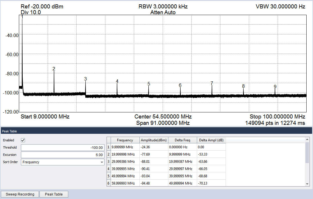
Peak table measuring the harmonics of a 10MHz input CW signal.
Real-Time Spectrum Analysis
All Signal Hound spectrum analyzers can operate as real-time spectrum analyzers. Real-time spectrum analysis is enabled by selecting Analysis Mode > Real Time in the main menu. In this mode, bandwidth is limited to the real-time bandwidth, which varies by device.
Real-time analysis is critical for characterizing short-duration spectral events such as spurious emissions or interference. It is also well suited for monitoring spread spectrum signals and frequency hopping communications channels.
Real-time spectrum analysis guarantees 100% probability of intercept for signals exceeding a minimum duration. That duration depends on the Signal Hound spectrum analyzer and the resolution bandwidth — any signal that exceeds it is guaranteed to be captured and displayed by Spike.
When in real-time mode, a special persistence display is shown. The persistence display presents a three-dimensional view of signal density over the configured span, where the X and Y axes show amplitude over frequency and color represents signal density at each point. As density increases, the color transitions from blue to green to red. Signal Hound spectrum analyzers can generate these plots from thousands to over a million traces per second depending on RBW. The persistence display accumulates approximately 2/3 of a second of real-time data.
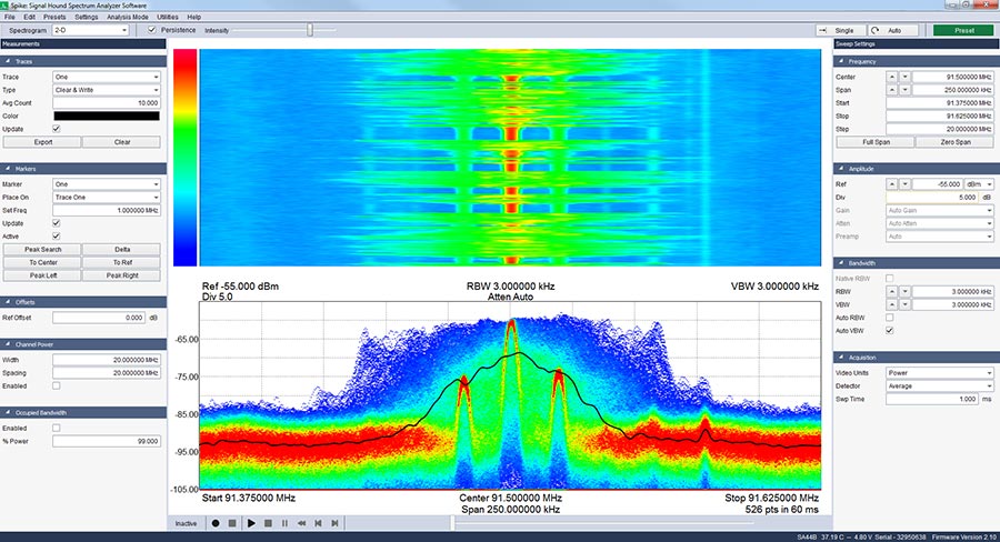
SA44B measuring an FM signal in real-time mode. A spectrogram display is shown in the upper half, and the persistence display in the lower.
Control Panels
Real-time spectrum analysis shares control panels with standard spectrum analysis. See Swept Analysis for more information.
I/Q Analysis (Zero-Span)
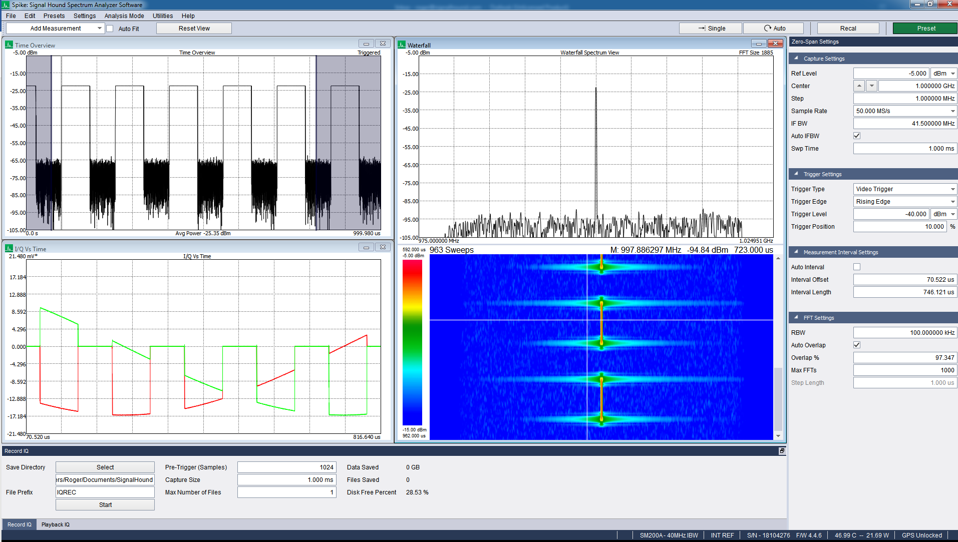
Triggering on a pulsed waveform in zero-span mode.
Zero-span analysis allows a user to view and analyze complex signals in the time domain. The application can demodulate AM, FM, and PM modulation schemes and display the results through multiple configurable plots. Enter zero-span mode via the Analysis Mode drop-down menu or by pressing the Zero Span button on the Sweep Settings control panel.
The control panel provides inputs for controlling capture settings and specifying trigger conditions. Available triggers are video and external. Video triggers begin the sweep once a signal exceeds the specified amplitude. External triggering begins acquisition when a signal is detected on the spectrum analyzer's trigger input port.
The control panel also includes a section for defining the measurement interval — a subset of the zero-span capture visible across the various plots. The Time Overview plot shows the interval relative to the whole capture and provides a graphical interface for adjusting the same parameters.
Zero-span mode supports recording and playback of I/Q waveforms via the record and playback control panels. See Zero-Span Recordings for details.
Zero-Span Settings Control Panel
Capture Settings
- Ref Level – Expected input power of the signal. Controls the reference level, gain, and attenuation. It is recommended to keep gain and attenuation set to Auto.
- Center – Specifies the tuned center frequency of the capture (the 0 Hz frequency of the I/Q data capture).
- Step – Controls how much the center frequency shifts when pressing the center frequency arrow keys or using the up/down keyboard arrows when the center frequency field is highlighted.
- Decimation – Controls the overall decimation of the I/Q data capture. A decimation of 2 divides the analyzer sample rate by 2. Increasing decimation increases possible capture time but decreases time resolution.
- Sample Rate – Displays the sample rate of the current visible I/Q data capture. Equal to the device sample rate divided by the decimation value.
- IF BW – (Intermediate Frequency Bandwidth) Controls the bandwidth of the passband filter applied to the I/Q data stream. Cannot exceed the Nyquist frequency of the I/Q data stream.
- Auto IFBW – When set to Auto, the IF bandwidth passes the entire bandwidth of the I/Q data capture.
- Swp Time – (Sweep Time) Controls the length of the zero-span data capture, relative to the sample rate set by decimation. Sweep times are clamped at a minimum when the capture contains fewer than 20 samples, and at a maximum when it contains more than 65,536 samples.
Trigger Settings
- Trigger Type – Select a trigger type for the data capture:
- Immediate – Acquisition begins immediately.
- Video – Triggers once sample amplitude crosses the user-specified trigger level.
- External – Triggers when a signal event is detected on the external trigger input port. Not available on all Signal Hound spectrum analyzers.
- Frequency Mask Trigger – See Frequency Mask Triggering for more information.
- Trigger Edge – Select whether to trigger on a rising or falling edge. Applies to both external and video triggers.
- Video Trigger – Set the amplitude for the video trigger. Ignored if video triggering is not selected.
- Trigger Position – When video or external trigger is selected, determines the percentage of samples displayed before the trigger. For example, in a 100-point sweep with a 10% trigger position, 10 points before and 90 points after the trigger are shown.
- Edit FMT – Open the frequency mask trigger editor dialog. See Frequency Mask Triggering for more information.
Measurement Interval Settings
Controls the measurement interval — the subset of the full capture displayed by all plots except Time Overview and Waterfall.
- Auto Interval – When enabled, the measurement interval spans the entire capture.
- Interval Offset – The time into the capture at which the measurement interval starts.
- Interval Length – The length of the measurement interval.
FFT Settings
Controls the FFT parameters for the spectrum and waterfall plots.
- RBW – The desired RBW for the spectrum plot. Lower RBWs increase the required FFT window length. If the window length is insufficient for the desired RBW, the spectrum window will show a warning. Increase the RBW, the FFT window length, or the overall capture size to resolve it.
- Auto Overlap – When enabled, an overlap percentage is chosen to produce the maximum number of FFTs up to Max FFTs.
- Overlap % – The percentage of overlap between FFTs.
- Max FFTs – The maximum number of FFTs. Computation stops when this number is reached, even if only part of the capture has been processed.
- Step Length – The time between the start of one FFT and the start of the next.
Record / Playback I/Q Control Panels
See Zero-Span Recordings.
Frequency Mask Triggering
Frequency mask triggering (FMT) is available in zero-span measurement mode. FMT takes overlapping FFTs on the input I/Q data and checks each result against a user-defined frequency mask. When FFT results exceed the mask, the software triggers acquisition starting at the beginning of the exceeding FFT. The FFT size is based on the current RBW with 50% overlap. A flat-top window is used for all spectrum processing in zero-span mode.
The frequency mask is configured using the FMT editor, which mirrors the standard zero-span spectrum plot as a guide. Using the editor buttons, you can add or remove mask points, create a mask from the spectrum plot as a baseline, apply frequency and amplitude offsets, and import or export existing masks. Each mask point can also be dragged directly on the spectrum plot using the left mouse button. Select OK to apply the mask — changes are not applied until OK is pressed.
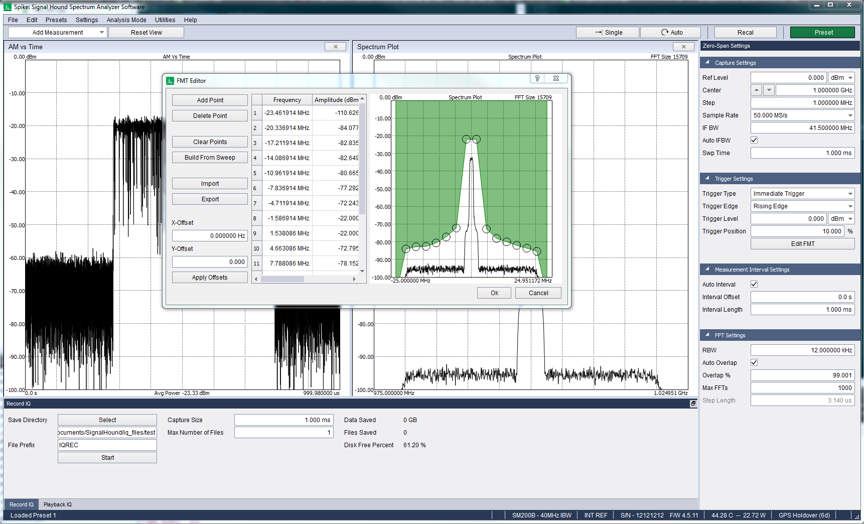
Frequency mask trigger editor
Zero Span Toolbar
Controls available in zero-span measurement mode:
- Add Measurement – Add a new measurement plot to the view area.
- Auto Fit – When selected, visible views are auto-scaled to fit the available application space. Disabling Auto Fit allows custom scaling and arrangement of views.
- Reset View – Resets the view area to the default configuration.
Zero-Span Plots
All plots in zero-span follow the Basic Plot interface in Spike.
Time Overview
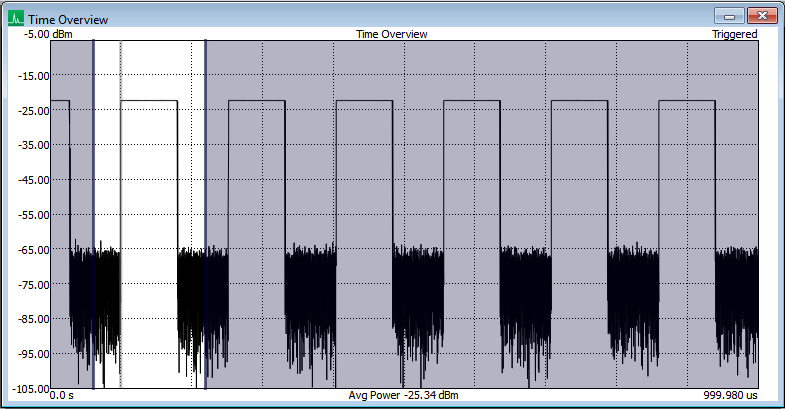
Time overview plot with the measurement interval set to encompass a triggered pulse
Shows and allows adjustment of the measurement interval relative to the whole capture. The measurement interval is the portion of the capture displayed by all other plots (except Waterfall, which shows all computed FFTs across the capture). The interval is represented by the unshaded region and can be adjusted by dragging it or its start/end points.
AM vs Time
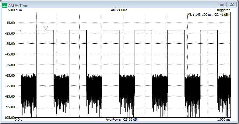
AM vs time plot on a triggered waveform
Shows the AM waveform over time. Supports log (dBm) or linear (mV) y-axis units. When triggering is enabled, a vertical gray bar appears at the trigger location. When spectrum acquisition is set to manual, a gray shaded region covers the selected FFT region. I/Q values can be exported by right-clicking and selecting Export I/Q (.csv).
FM vs Time
Plots the waveform as frequency vs. time.
PM vs Time
Plots the waveform as phase vs. time. Y-axis units can be set to radians or degrees.
I/Q vs Time
Plots the individual I and Q channels as amplitude in mV vs. time.
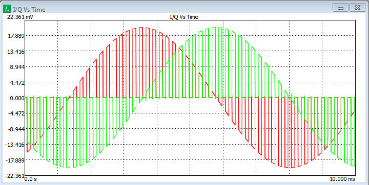
I/Q vs time plot of a pulsed CW signal
I/Q Polar Plot
Plots I/Q values as mV on the Cartesian plane. The plot scale is set to the selected reference level of the acquisition.
Spectrum Plot
Shows the frequency spectrum of the portion of the zero-span capture defined by the measurement interval. RBW is selectable up to the maximum number of points in the sweep (configured under FFT Settings). A flat-top window is used with zero-padding to achieve the selected RBW. All FFTs that form this plot must begin and end within the measurement interval, so the interval must be at least one FFT in length. If the selected RBW cannot be met with the current interval size, a warning message displays the required capture time.
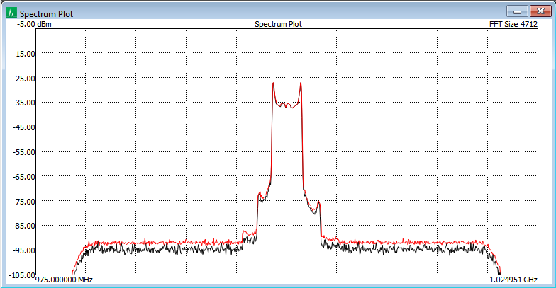
Spectrum plot of an FM signal with the max hold trace enabled.
CCDF Plot
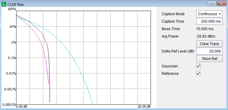
CCDF plot comparing synthetic noise to a Gaussian reference and ideal test signal.
The Complementary Cumulative Distribution Function (CCDF) plot shows how often the signal exceeds the average signal power. The x-axis runs from 0 dB above the signal mean to a user-selected reference level; the y-axis is the percentage of time the signal appears above a given amplitude.
The plot can operate on a single I/Q capture or a continuous series. In continuous mode, the capture time control sets the buffer size — new samples shift in as old samples shift out. A Gaussian reference curve representing the ideal Gaussian distribution can be overlaid. A user-stored reference waveform can be saved by pressing Store Ref, which stores the active trace in memory until pressed again.
Waterfall Plot
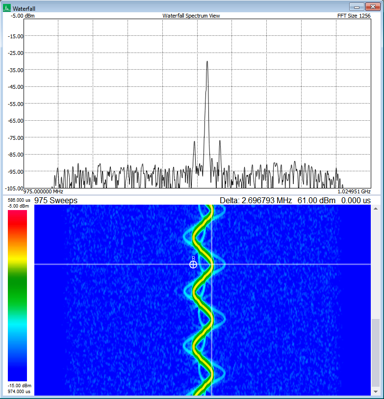
Waterfall plot measuring the deviation of an FM signal using the reference marker and a spectrum view of the peak.
Shows the frequency spectrum of the signal over time. When an FFT sweep is selected with the marker, it is shown in the Waterfall Spectrum View above the main plot. The Spectrum View can be enabled and disabled from the context menu preferences. This plot is functionally equivalent to the Spectrogram.
Channel Power Plot
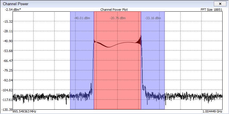
Channel power plot measuring the main and adjacent channels of an FM signal.
Configures and measures the channel power of a main channel and an optional adjacent channel (lower and upper components). The plot is created by averaging FFTs across the measurement interval and performing channel power measurements on the resulting spectrum. FFTs default to 50% overlap but spread out if needed to keep the FFT count at the configured maximum within the interval.
The configuration dialog is accessed through the context menu and allows setting the main channel width, enabling the adjacent channel with its width and offset, and setting the maximum number of FFTs. Widths and offsets default to ¼ of the sample rate with 100 max FFTs.
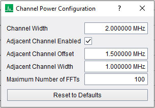
Channel power plot configuration dialog.
Zero-Span Recordings
WARNING: Zero-span recording can consume a large amount of hard drive space in a short time. Exercise caution, particularly when storing waveforms on the Windows system drive.
In zero-span mode, users can save and play back short-duration I/Q waveforms. Waveforms are recorded in SigMF© format. For long-term I/Q recording, see I/Q Recorder.
Recording
I/Q captures are performed using the Record I/Q control panel. Settings:
- Save Directory – The default directory for storing I/Q waveform files.
- File Prefix – Applies a prefix to all saved file names, useful for creating identifiable files.
- Capture Size – Specify the minimum capture length for a single file.
- Max Number of Files – Specify the number of waveforms to record.
Press Start to begin acquisition. If the trigger type is No Trigger, acquisition begins immediately. With external or video trigger, the software waits for a trigger event. When saving more than one file with an active trigger, each file requires its own trigger to start. Plots do not update during acquisition, but status statistics and remaining disk capacity are displayed.
Playback
A recorded file can be viewed using the Playback I/Q control panel. Press Open File and select the metadata file for the capture to view. Playback begins immediately.
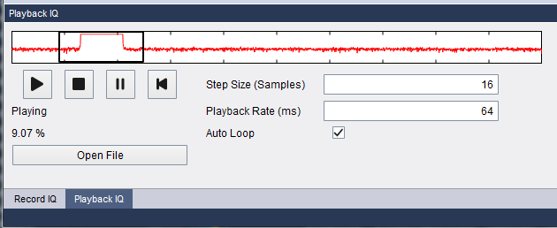
I/Q playback control panel.
Tools available during playback:
- I/Q scroll bar – Provides a preview trace of the full capture and a selectable region for quickly navigating the waveform.
- Step size – Specifies the number of samples to advance on each view update. Only applicable when no triggering is active.
- Playback rate – Controls the speed at which Spike updates when loading waveforms from the file.
- Single/Auto buttons – Use to step through the capture manually.
- Video Trigger – Forces Spike to search the capture for a trigger before updating plots. If no trigger is found, playback stops at the end of the file.
To begin playback: press Open File, ensure the Playing message is shown, and press Auto in the toolbar with No Trigger selected. The view window in the scroll bar will advance to the right as the file is read. Press Single at any time to pause and step through manually. Dragging the scroll bar view window to a new position pauses playback — press Play to resume.
If the Playing message is shown but the waveform is not updating, ensure you are not in single trigger mode. Searching for a trigger in a very large file may cause a delay of several seconds — use the scrollbar to navigate to the region of interest or record smaller files to reduce this delay.
I/Q File Format
Each I/Q capture uses the SigMF© format, which consists of one metadata file and one data file. Spike records and processes only the first capture per file.
The metadata file contains acquisition settings and scale factors needed to reconstruct the original I/Q waveform. Metadata fields:
- core:hw – Product name of the analyzer used in the acquisition.
- core:datatype – Should be Complex Short, indicating the binary format of the I/Q data file.
- core:sample_rate – Sample rate in Hz of the I/Q waveform acquisition.
- core:datetime – ISO 8601 datetime string with nanosecond precision. References the first sample in the acquisition.
- signalhound:reference – The reference level in dBm set in Spike for the acquisition.
- signalhound:bandwidth – Cutoff frequency of the I/Q bandpass filter.
- signalhound:scale – Used to scale the I/Q data from full scale to mW.
- signalhound:preview – Values used to create the waveform trace on the I/Q playback scroll bar, generated via max-hold decimation on the full capture.
The binary data file contains signed 16-bit I/Q values in little-endian byte order, stored sequentially as:
I1, Q1, I2, Q2 … In, Qn
Values range from -32768 to +32767, representing floating-point values from -1.0 to +1.0. To recover the original values:
- Read the binary file into signed 16-bit complex values.
- Convert the 16-bit I and Q integers to floating-point values in the range [-1.0, +1.0].
- Multiply each I and Q value by the inverse of the scale factor from the metadata file.
- I/Q samples are now scaled to mW, where I² + Q² = mW.
I/Q Capture: Precautions
- Store waveforms to an external hard drive rather than the OS drive. If the OS drive approaches 100% capacity, it may prevent the OS from operating properly. If storing on the OS drive is unavoidable, keep at least 20% free (Windows recommends 15%).
Calculate expected capture size beforehand:
Size of Capture (Bytes) = Sample Rate (S/s) × Capture Time (s) × 4
Example: a 5-second capture with a BB60C at full sample rate = 40 MS/s × 5 × 4 = 800 MB
Ensure hard drive write speed exceeds the acquisition speed:
Write Speed (Bytes/s) = Sample Rate × 4
For the highest BB and SM series sample rates, a solid-state drive and/or RAID configuration may be necessary.
- When capturing multiple triggered events over an extended interval, perform test runs on known signals first to verify acquisition settings before committing to a long session.
I/Q Analysis (Multi-Channel)
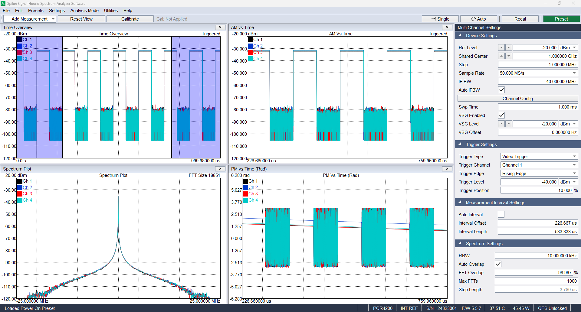
Triggering on and measuring a pulsed waveform in multi-channel I/Q analysis.
Multi-channel analysis allows users to view and analyze complex signals in the time domain. The application can demodulate AM and PM modulation schemes and display the results through multiple configurable plots. Enter multi-channel mode via the Analysis Mode drop-down menu or by pressing the Multi-Channel Analysis button.
The control panel provides inputs for controlling capture settings and specifying trigger conditions. Available triggers are video and external. Video triggers begin the sweep once a signal exceeds the specified amplitude. External triggering begins acquisition when a signal is detected on the trigger input port.
The control panel also includes a section for defining the measurement interval — a subset of the multi-channel capture visible across the various plots. The Time Overview plot shows the interval relative to the whole capture and provides a graphical interface for adjusting the parameters. Multi-channel mode currently offers six unique plots.
Multi-Channel Settings Control Panel
Device Settings
- Ref Level – Expected input power of the signal. Controls gain and attenuation. It is recommended to keep gain and attenuation set to Auto.
- Shared Center – Specifies the tuned center frequency of the capture (the 0 Hz frequency of the I/Q data capture).
- Channel Config – Opens the channel configuration dialog:
- Enabled – Enable or disable the specified channel.
- Use Independent LO – Enable the independent LO for the specified channel.
- Independent Center – Specifies the tuned center frequency using the independent LO for that channel.
- Step – Controls the center frequency shift when pressing the arrow keys or keyboard up/down arrows while the center frequency field is highlighted.
- Sample Rate – Displays the sample rate of the current visible I/Q data capture. Equal to the device sample rate divided by the decimation value.
- IF BW – (Intermediate Frequency Bandwidth) Controls the bandwidth of the passband filter applied to the I/Q data stream. Cannot exceed the Nyquist frequency of the I/Q data stream.
- Auto IFBW – When set to Auto, the IF bandwidth passes the entire bandwidth of the I/Q data capture.
- Swp Time – (Sweep Time) Controls the length of the data capture, relative to the sample rate. Sweep times are clamped when the capture contains fewer than 20 samples or more than 65,536 samples.
- VSG Enabled – Used to enable the VSG.
- VSG Level – Expected output power of the VSG signal.
- VSG Offset – Offset frequency of the VSG signal. The VSG uses the shared LO, so this offset is relative to the Shared Center.
Trigger Settings
- Trigger Type – Select a trigger type for the data capture:
- Immediate – Acquisition begins immediately.
- Video – Triggers once sample amplitude crosses the user-specified trigger level.
- External – Triggers when a signal event is detected on the external trigger input port. Not available on all Signal Hound spectrum analyzers.
- Trigger Channel – Select the channel to trigger from when trigger type is Video. Greyed out if video triggering is not selected.
- Trigger Edge – Select whether to trigger on a rising or falling edge. Applies to both external and video triggers.
- Trigger Level – Set the amplitude for the video trigger. Ignored if video triggering is not selected.
- Trigger Position – When video or external trigger is selected, determines the percentage of samples displayed before the trigger. For example, in a 100-point sweep with a 10% trigger position, 10 points before and 90 points after the trigger are shown.
Measurement Interval Settings
Controls the measurement interval — the subset of the full capture displayed by all plots except Time Overview and Waterfall.
- Auto Interval – When enabled, the measurement interval spans the entire capture.
- Interval Offset – The time into the capture at which the measurement interval starts.
- Interval Length – The length of the measurement interval.
FFT Settings
Controls the FFT parameters for the spectrum and waterfall plots.
- RBW – The desired RBW for the spectrum plot. Lower RBWs increase the required FFT window length. If the window length is insufficient for the desired RBW, a warning is shown. Increase the RBW, the FFT window length, or the overall capture size to resolve it.
- Auto Overlap – When enabled, an overlap percentage is chosen to produce the maximum number of FFTs up to Max FFTs.
- Overlap % – The percentage of overlap between FFTs.
- Max FFTs – The maximum number of FFTs. Computation stops when this number is reached, even if only part of the capture has been processed.
- Step Length – The time between the start of one FFT and the start of the next.
Multi-Channel Toolbar
Controls available in multi-channel measurement mode:
- Add Measurement – Add a new measurement plot to the view area.
- Reset View – Resets the view area to the default configuration.
- Calibrate – Opens the Calibration Dialog. See Multi-Channel Calibration.
- Cal Status – Displays the current calibration status:
- Cal: Not Applied – No calibration has been applied.
- Cal: Applied (Exact) – A calibration is applied and was collected at the exact frequency the device is currently tuned to.
- Cal: Applied (Interpolated) – A calibration is applied based on linear interpolation between two calibration points, as the device is not tuned to an exact calibrated frequency.
Multi-Channel Plots
All plots in multi-channel follow the Basic Plot interface in Spike, except for the markers.
Multi-Channel Markers
Markers can be placed on the nearest x-axis point for each active graph by left-clicking. For time-domain plots, markers are shared between plots. Use the left/right arrow keys to move a marker one index at a time. When a marker is active, selecting Delta Marker from the context menu places a reference marker at the current location; selecting it again disables the delta marker.
The marker readout includes a channel-to-channel delta for quick phase and amplitude comparisons between channels.
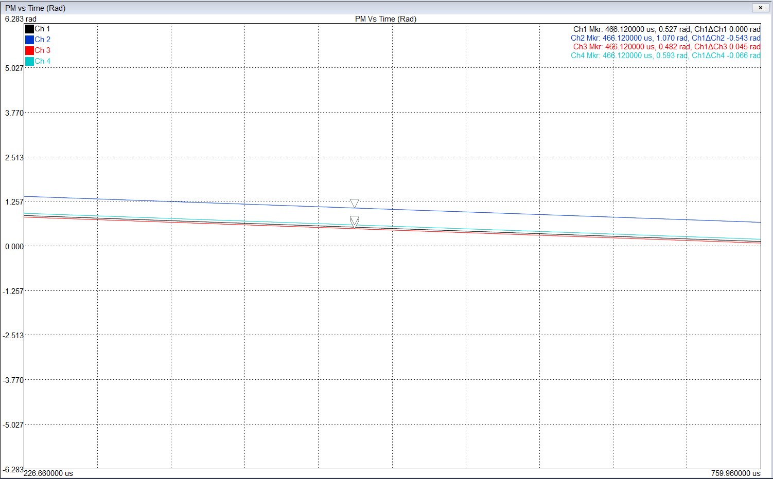
Multi-channel markers on a PM vs time plot.
Time Overview
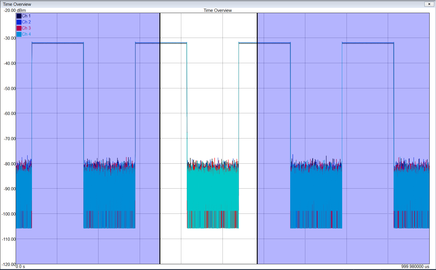
Time overview plot with the measurement interval over a triggered pulse.
Shows and allows adjustment of the measurement interval relative to the whole capture. The measurement interval is the portion of the capture displayed by all other plots (except Waterfall, which shows all computed FFTs across the capture). The interval is represented by the unshaded region and can be adjusted by dragging it or its start/end points.
AM vs Time
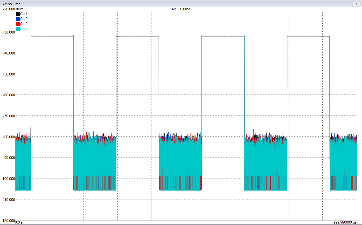
AM vs time plot on a triggered waveform.
Shows the AM waveform over time. Supports log (dBm) or linear (mV) y-axis units. When triggering is enabled, a vertical gray bar appears at the trigger location. When spectrum acquisition is set to manual, a gray shaded region covers the selected FFT region. I/Q values can be exported by right-clicking and selecting Export I/Q (.csv).
PM vs Time (Rad)
Plots the waveform as phase in radians vs. time.
Phase Delta vs Time
Plots the waveform as phase in radians vs. time for all channels relative to the lowest active channel.
Spectrum Plot
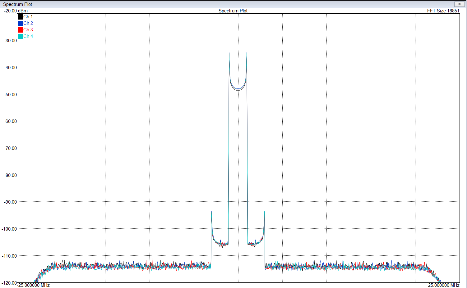
Multi-channel spectrum plot of an FM signal with 1MHz frequency deviation.
Shows the frequency spectrum of the portion of the multi-channel capture defined by the measurement interval. RBW is selectable up to the maximum number of points in the sweep (configured under FFT Settings). A flat-top window is used with zero-padding to achieve the selected RBW. All FFTs forming this plot must begin and end within the measurement interval — the interval must be at least one FFT in length. If the selected RBW cannot be met with the current interval size, a warning displays the required capture time.
Waterfall Plot
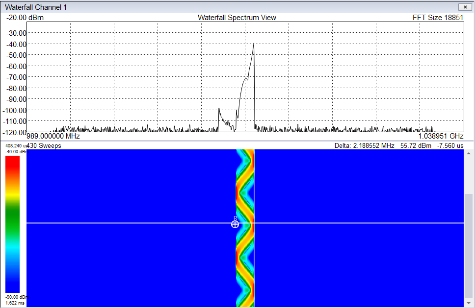
Measuring deviation of FM signal using reference marker and a spectrum plot to observe the peak.
Shows the frequency spectrum of the signal over time. When an FFT sweep is selected with the marker, it is shown in the Waterfall Spectrum View above. The Spectrum View can be enabled and disabled from the context menu preferences. The displayed channel can be selected via Channel Selection in the context menu. This plot is functionally equivalent to the Spectrogram.
Multi-Channel Calibration
Multi-channel calibration provides a mechanism for calibrating channel-to-channel amplitude, phase delay, and phase offset. All corrections are collected with reference to channel 1.
Calibration Setup
The standard setup requires a 4-channel splitter and 5 cables of equal length. Connect the PCR4200's VSG to the input of the splitter and each output to one of the PCR4200 channels.
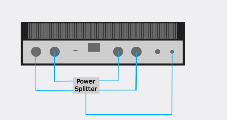
PCR4200 calibration setup.
Calibration Dialog
Opened via the Calibrate button in the Multi-Channel Toolbar. Includes a graph displaying the currently selected corrections.
- View – Select which corrections to display on the graph.
- Load Calibration – Opens a file dialog to select a calibration file to load.
- Unload Calibration – Unloads the currently loaded calibration.
- Perform Calibration – Opens the Perform Calibration Dialog.
- Status – Displays the number of points in the current calibration, or "No calibration loaded."
- File – Name of the currently loaded calibration file.
- Temperature – Device temperature in °C at the time the current calibration was performed.
- Calibrated – Date and time at which the current calibration was performed.
- Setup – Short description of the hardware setup used for the current calibration.
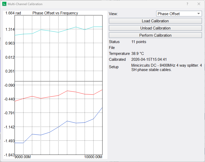
Multi-channel calibration dialog with a currently loaded calibration.
Perform Calibration Dialog
Used to configure and run a calibration. Includes an image of the typical hardware setup. When calibration completes, you are prompted to save the file (extension: .shmccal).
- Setup Description – Short description of the hardware setup for this calibration.
- Start Freq – First frequency step of the calibration.
- Stop Freq – Final frequency step of the calibration.
- Step Freq – Step size used to form the calibration.
- Calibrate – Starts the calibration.
- Cancel – Cancels a calibration in progress.
- Cal Points – The number of points in the calibration.
- Progress – Shows calibration progress as a percentage.
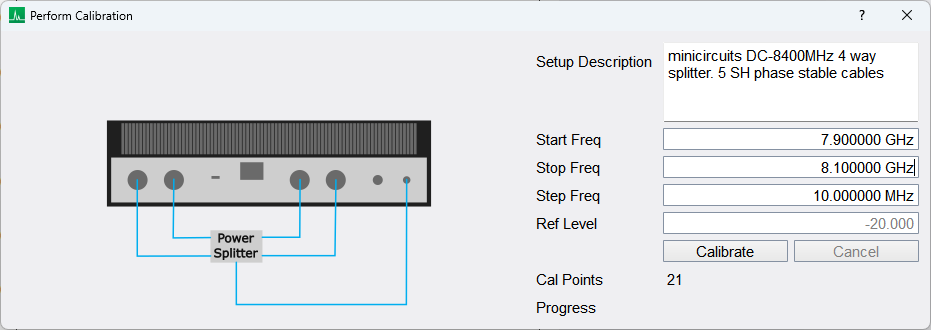
Multi-channel calibration dialog.
Harmonic Analysis
The harmonic measurement mode measures up to 10 harmonics of a specified carrier frequency. Each measurement consists of a sweep at the fundamental and all harmonic frequencies. Span, RBW, and VBW are configurable. All harmonic sweeps are plotted sequentially and amplitudes are reported as dBc. Total harmonic distortion (THD) is displayed in the upper right-hand corner of the spectrum plot.
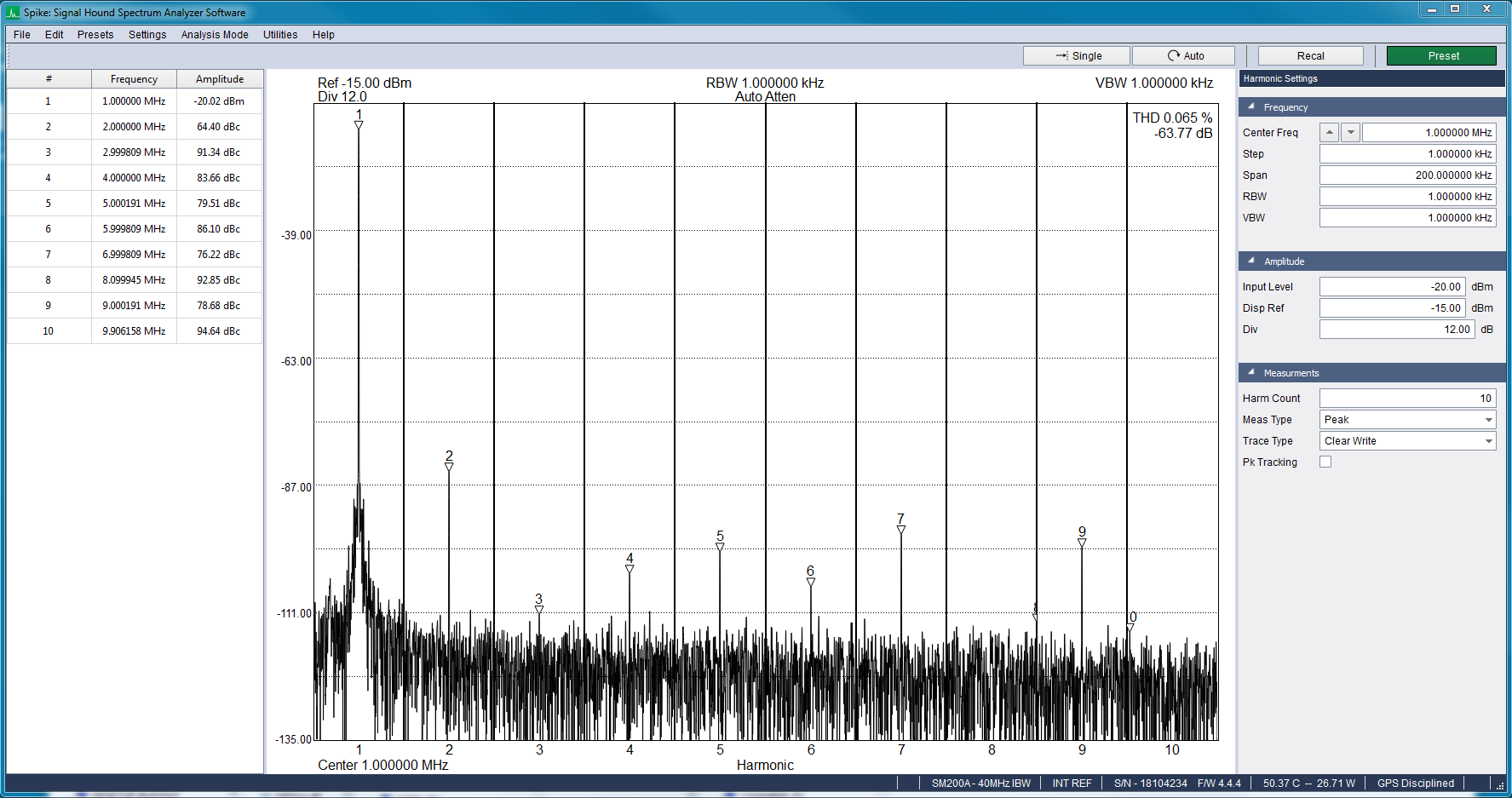
Harmonic analysis on a carrier frequency at 1MHz, measuring out to 9 harmonics.
Measurement Analysis Procedure
The first sweep is performed centered at the selected Center Freq. If peak tracking is enabled, the center frequency used is the previously measured fundamental frequency. The frequency and amplitude of the fundamental are measured using either a peak search or channel power, depending on the Meas Type selection. When channel power is selected, frequency is determined by the center of the 90% occupied bandwidth.
All subsequent harmonics are measured at multiples of the measured fundamental frequency, stored as dBc. The spectrum plot and harmonic list update as each harmonic measurement is performed. Measuring and plotting all harmonics constitutes a single measurement.
Harmonic Analysis Controls
- Center Freq – The center frequency of the fundamental measurement.
- Step – Controls the frequency step of the arrows on the Center Freq control.
- Span – The measurement span used at each harmonic.
- RBW – The measurement RBW used at each harmonic.
- VBW – The measurement VBW used at each harmonic.
- Ref Level – The maximum expected input level. Recommended to set 5 dB above the maximum expected input.
- Disp Ref – The displayed reference level of the spectrum plot.
- Div – Vertical spectrum plot division height.
- Harm Count – Number of harmonics to measure and plot.
- Meas Type – Select the measurement type at each harmonic. Peak performs a peak search to find frequency and amplitude. Channel Power uses a channel power measurement for amplitude and an occupied bandwidth measurement for frequency.
- Trace Type – Select the trace behavior.
- Pk Tracking – When enabled, the fundamental is measured at the previously measured fundamental frequency. Resets to the selected Center Freq whenever any setting is changed.
Scalar Network Analysis
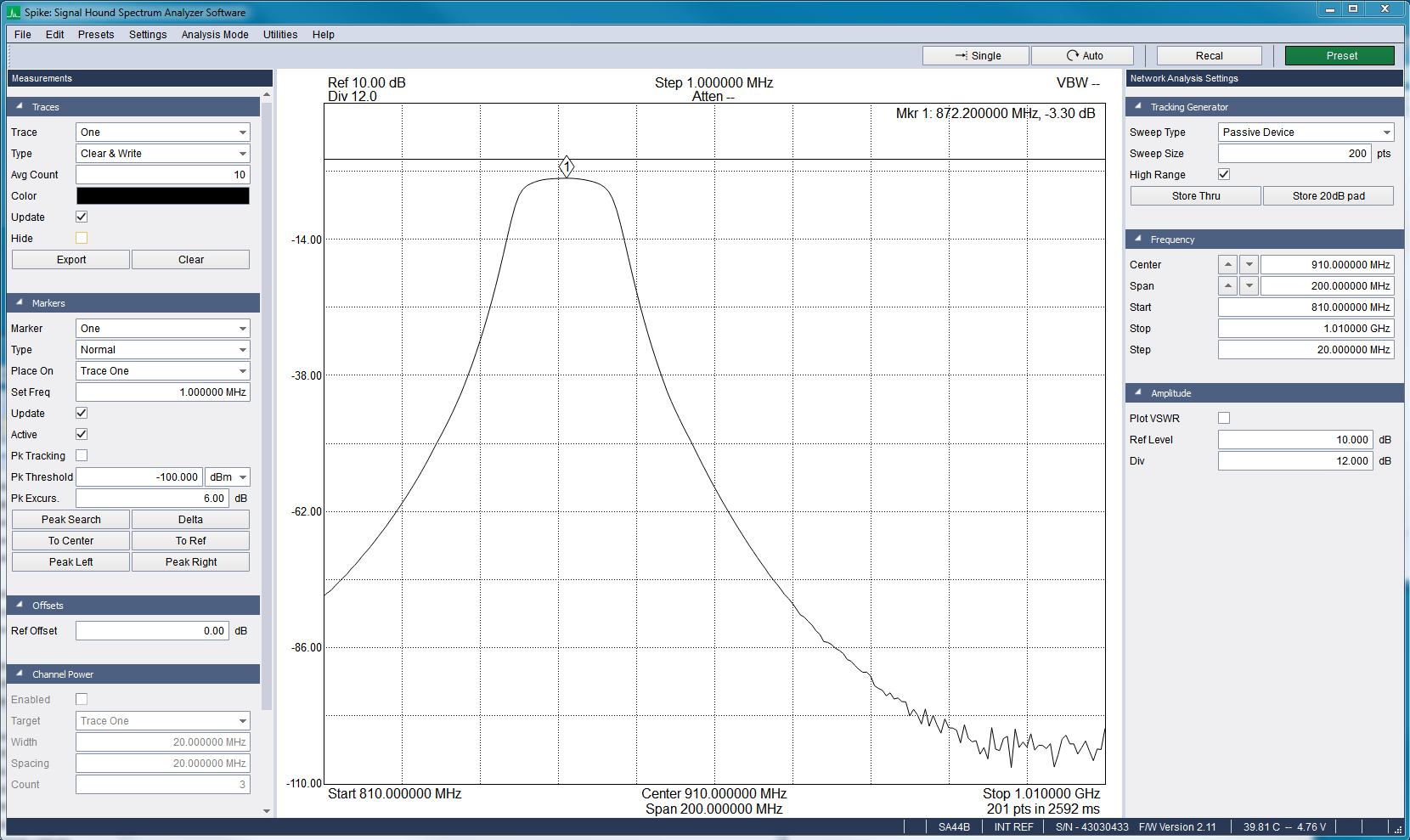
Scalar network analysis of a bandpass filter using the SA44B and TG44A.
If a BB or SA-series spectrum analyzer and a compatible tracking generator are both connected to the PC, select Analysis Mode > Scalar Network Analysis. This mode measures the insertion loss of a device such as a filter, attenuator, or amplifier across a range of frequencies. When used with a directional coupler, it can also measure return loss.
Ensure the TG sync port on the tracking generator is connected to the Sync Out port on the SA series spectrum analyzer. For more information, refer to the Signal Hound Tracking Generator user manual.
Scalar Network Analysis Control Panel
Tracking Generator Settings
- Sweep Type – Specify whether an active or passive device is being swept. This affects the attenuation and gain used during the sweep. Incorrect selection may reduce dynamic range or cause IF overload.
- Sweep Size – Specify a suggested sweep size. Final sweep size is also affected by hardware limitations.
- High Range – When selected, the software optimizes for dynamic range when a 20 dB pad store-through is performed. Deselecting increases sweep speed at the cost of dynamic range.
- Store Thru – Press to normalize the sweep on the next acquired sweep. Can be re-pressed if a poor normalization occurred.
- Store 20dB Pad – Perform a normalization with a 20 dB pad inserted in the RF path. Should only be performed after a normal Store Thru.
Frequency Settings
- Center – Specify the center frequency of the sweep. Span will be reduced if start or stop frequencies fall outside the device's operating range. Arrows change the center frequency by the step amount.
- Span – Specify the frequency difference between start and stop frequencies. Span is reduced if it causes frequencies to fall outside the operating range. Arrows change the span using a 1/2/5/10 sequence.
- Start/Stop – Specify the start and stop frequencies. Frequencies outside the operating range of the active device cannot be selected.
- Step – Specify the step size for the center frequency arrows.
Amplitude Settings
- Plot VSWR – Plot return loss as VSWR.
- Ref Level – Specify the displayed reference level. Changing this updates the display immediately without affecting calibration status. Specified in dB or SWR depending on whether Plot VSWR is selected.
- Div – Specify the vertical plot divisions. When plotting VSWR, the graticule ranges from 1.0 at the bottom to 1.0 + 10 × div at the top. On a log scale, it ranges from Ref Level at the top to Ref Level – 10 × div at the bottom.
Measurements Control Panel
See Measurements Control Panel in Swept Analysis mode.
Configuring Scalar Network Analyzer Sweeps
- Use the Frequency controls to set the desired center frequency and span.
- For most devices, a start frequency > 250 kHz and span > 100 kHz is recommended for maximum dynamic range, sweep speed, and accuracy.
- (SA44/SA124 only) For crystals or high-Q circuits with bandwidths of 50 Hz to 10 kHz, select a span ≤ 100 kHz. A slower narrow-band mode activates automatically; a 100-point sweep takes approximately 7 seconds but updates at each point.
- Use the Amplitude controls to set the Reference Level. A good starting value is +10 dB.
- Use the Tracking Generator Controls:
- Select the desired sweep size (100 points is a good starting point).
- Select Active Device if measuring an amplifier.
- Leave High Range checked unless faster sweeps are needed at the cost of dynamic range.
- For accurate measurements below -45 dB, use the defaults of Passive Device and High Range.
Performing Sweeps
Before measurements can be made, a baseline (0 dB insertion loss reference) must be established using Store Thru:
- Connect the tracking generator RF output directly to the spectrum analyzer RF input.
- Click Store Thru and wait for the sweep to complete. The sweep normalizes to 0 dB. Readings from 0 dB to approximately -45 dB are now calibrated.
- (Optional) For accurate measurements below -45 dB, insert a fixed SMA attenuator (at least 16 dB, no more than 32 dB) and click Store 20 dB Pad. This corrects offsets between high and low range sweeps, giving accurate readings down to the noise floor.
- Insert the device under test (DUT) between the tracking generator and spectrum analyzer and take measurements. All traces and markers are accessible during network analyzer sweeps.
Note: Changing sweep settings (frequency, amplitude, etc.) requires repeating steps 1–4.
Improving Accuracy
Adding quality 3 dB or 6 dB SMA attenuators (pads) to the tracking generator output and/or spectrum analyzer input significantly improves return loss performance. A 6 dB pad typically improves return loss by ~12 dB to >20 dB. Include the pads during the Store Thru sweep to null them out — this reduces overall dynamic range slightly.
Testing High Gain Amplifiers
When measuring an amplifier with 20–40 dB of gain, a 20 dB pad is required. Insert the pad before Store Thru and leave it in the signal chain when connecting the amplifier. Place the pad on the amplifier output for amplifiers with > +20 dBm maximum output, or on the amplifier input if the amplifier cannot safely handle -5 dBm.
Measuring Return Loss
- Connect the tracking generator to the directional coupler's OUT port.
- Connect the spectrum analyzer to the directional coupler's COUPLED port.
- Use the IN port as the test port, left open (reflecting 100% of power). If using a cable between the test port and antenna, connect the cable to IN but leave the far end open.
- Click Store Thru. The sweep normalizes to 0 dB.
- Connect the device under test (e.g., antenna) to the IN port. Return loss is plotted.
Adding 3–6 dB pads on the Signal Hound devices before Store Thru improves accuracy. With a good directional coupler, accuracy within a few tenths of a dB is typical.
Adjusting an Antenna
Use the return loss setup above. Lengthen, shorten, and tweak impedance matching elements until the desired return loss is achieved. Note that RF will be radiated during this process — ensure compliance with applicable transmit regulations.
Levels Used in Sweeps
- High Range disabled – The tracking generator sweeps at -30 dBm.
- High Range enabled – The tracking generator performs two sweeps: once at -30 dBm, then at -10 dBm. These are combined into a single measurement in Spike.
- Passive Device – The analyzer expects the signal at or below the tracking generator output power.
- Active Device – The analyzer allows up to 20 dB of amplification.
Exceeding the analyzer's expected input level can overload the analyzer and produce invalid measurements. Add an attenuator in the signal chain if additional gain reduction is needed.
Manual Tracking Generator Sweeps
For devices with bandwidths below 50 Hz (e.g., a 60 Hz notch filter) or when more than 90 dB of dynamic range is required, do not use Scalar Network Analysis mode. Instead, remain in Swept Analysis mode and use Utilities > Tracking Generator Controls to set the tracking generator to a CW frequency output. Use Peak Search and Delta to establish a relative amplitude reference, then insert the DUT and manually tune the TG across a narrow frequency range. A TG output of -10 dBm combined with an RBW of 10 Hz provides approximately 130 dB of dynamic range for most frequencies. Take care with cable and device placement to avoid crosstalk.
Phase Noise Measurements
The phase noise measurement mode measures the single-sideband (SSB) phase noise of an input RF signal. Phase noise can be measured using any single Signal Hound spectrum analyzer, or using the PN400 phase noise test system. For measurements with the PN400, see Cross-Correlation.
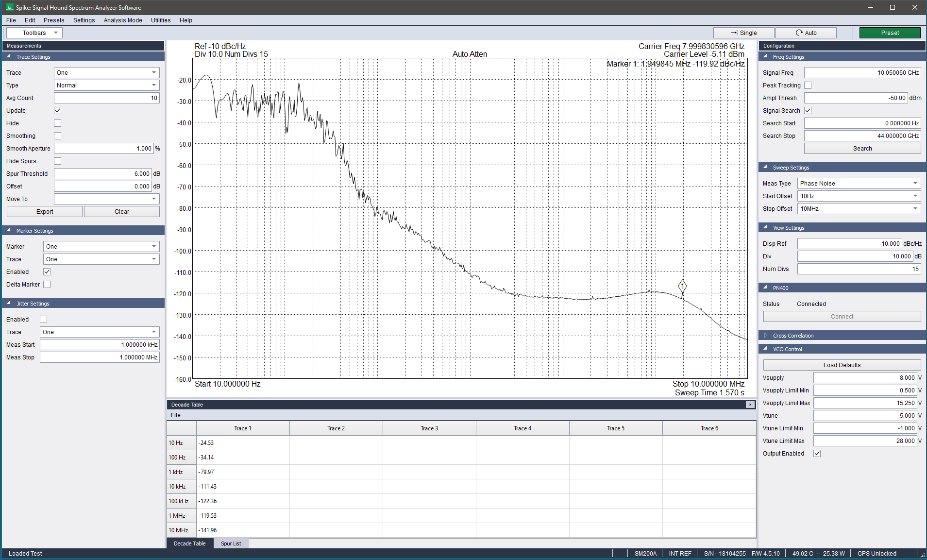
Phase noise measurement of a VCO at 8GHz using the SM200B.
Measurement Theory
This section describes phase noise measurements made with a single spectrum analyzer. The measurement requires a fixed CW input into the analyzer. If the input signal is removed at any point, measurement updates stop and a warning is displayed on the phase noise plot.
When configuring a new measurement, a coarse frequency estimate must be made. This can be determined automatically using the signal search function or entered manually in the carrier frequency setting. Once a coarse estimate is made, a fine frequency and amplitude estimate is performed to establish the measurement configuration. A fine estimate is performed prior to every phase noise measurement to ensure optimal settings are always used in the event of signal drift.
The phase noise measurement uses an FFT approach and can measure phase noise, AM noise, or both simultaneously. The resulting sweep contains 100 points per decade. Each result is used to update the user-configured traces and trace measurements.
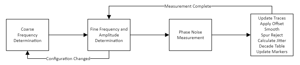
Measurement flow graph.
Cross-Correlation
Using the PN400 adapter and two SM200/435 spectrum analyzers, Spike can perform cross-correlated phase noise measurements, improving sensitivity by up to 35 dB over the base SM phase noise performance.
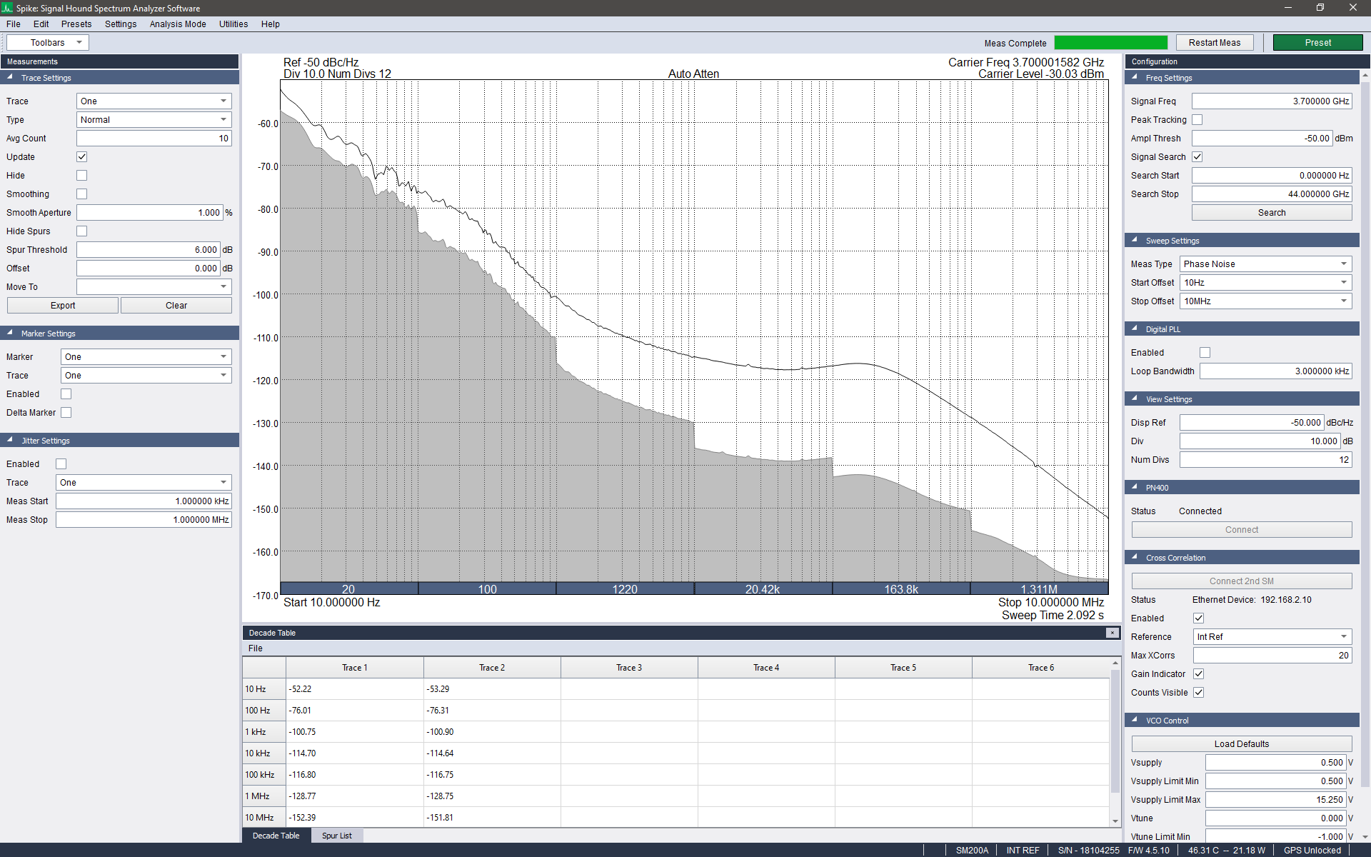
Cross correlation measurement at 3.7GHz.
To enable cross-correlation:
- Connect equipment according to the cross-correlation setup diagram. Optionally connect a shared 10 MHz reference (or a 10 MHz reference output from the DUT) to the 10 MHz reference input on the SM devices.
- In phase noise measurement mode, connect to both the PN400 and the second SM analyzer using the controls in the configuration control panel.
- (Optional) Configure VCO supply and tuning voltages if measuring a VCO.
- Enable cross-correlation.
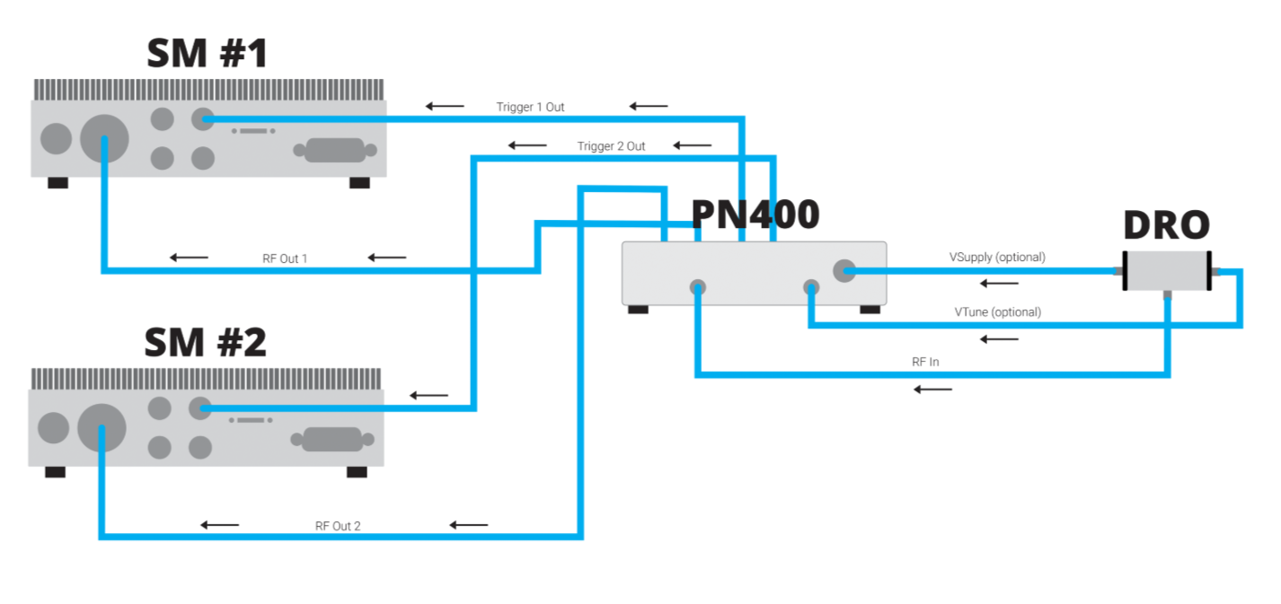
Typical cross-correlation setup using the PN400 adapter.
Measurement Theory
This section covers cross-correlated phase noise measurements. For non-correlated phase noise measurements, see Measurement Theory.
Cross-correlation improves phase noise measurement performance by making a simultaneous measurement on a second device and using signal processing to reduce the noise floor. More cross-correlations yield better improvement. Spike uses a direct FFT method that enables more correlations at wider offsets. The number of correlations is displayed per decade.
Performance improvement factor: 5 × log10(# of correlations)
| Correlation Count | Gain (dB) |
| 10 | 5 |
| 100 | 10 |
| 1,000 | 15 |
| 10,000 | 20 |
| 100,000 | 25 |
| 1,000,000 | 30 |
| 10,000,000 | 35 |
Once the maximum number of correlations is reached, the measurement stops and must be manually restarted. Any change to the measurement settings automatically restarts the measurement. Processing stops for a given offset once its maximum correlation count is reached, but continues for other offsets. Wider offsets reach maximum correlations faster than close-in offsets.
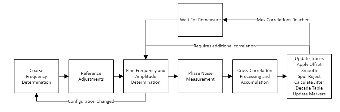
Cross-correlation measurement flow graph.
Reference
For best results, both SM analyzers should use the same reference clock. This setting overrides the Spike reference setting in Settings > Reference.
- Int Ref – Both devices use their internal 10 MHz references. A configuration step attempts to synchronize these clocks as closely as possible.
- Ext Ref – Both devices use an external 10 MHz reference, preferably shared with the DUT or provided directly by it.
- RF Ref – The input RF frequency disciplines the two SM devices. Signal search is bypassed and the entered Signal Freq is used directly.
Gain Indicator
The gain indicator is the gray region displayed below the trace when cross-correlation is enabled. It represents the ideal trace location if the full performance gain of cross-correlation were realized. If the gain indicator improves significantly faster than the measured trace — or the trace no longer improves — additional correlations are unlikely to provide further benefit. The user must determine how much separation is required to have confidence in the measurement.
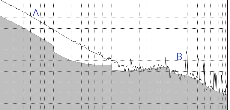
The separation near "A" indicates we are adequately measuring the DUT at this frequency offset. The lack of separation at "B" indicates either additional correlations are needed, or this measurement performance is out of range for this DUT, aka we are already at max correlations.
Measuring Near Cardinal Frequencies
Spurious signals can appear when measuring near or at 100 MHz multiples during cross-correlated phase noise measurements. Using an external reference shared between the SM devices and DUT, or selecting RF Ref, can reduce or eliminate these mixing spurs.
Phase Noise Control Panel
Frequency Settings
- Signal Freq – When signal search is disabled, this value is used for the coarse frequency estimate.
- Peak Tracking – When enabled, small drifts in signal frequency are tracked during the fine estimation procedure.
- Ampl Thresh – Specify the minimum detected carrier level required to perform a phase noise measurement. If not met, the software continues searching for a valid carrier.
- Signal Search – When enabled, the input frequency is estimated using a wideband sweep between the search start and stop frequencies. This can be time-consuming on slower devices; manually entering a known frequency is recommended when possible.
- Search Start – Start frequency for automatic signal search. Ignored if signal search is disabled.
- Search Stop – Stop frequency for automatic signal search. Ignored if signal search is disabled.
Sweep Settings
When using the SA44/SA124, start/stop offsets can drastically affect measurement speed. See Measurement Speed (SA44/SA124 only) for more information.
- Meas Type – Select whether to measure and display phase noise, amplitude noise, or both.
- Start Offset – Select the first decade to be measured and plotted.
- Stop Offset – Select the last decade to be measured and plotted.
View Settings
Controls the vertical range of the phase noise plot. Total vertical range: [Max, Min] = [DispRef, DispRef − Div × NumDivs]
- Disp Ref – Specify the displayed reference level in dBc/Hz.
- Div – Specify the plot division height in dB.
- Num Divs – Specify the number of vertical plot divisions.
PN400
Settings for connecting and controlling the PN400 accessory. Set voltage limits before setting voltages to prevent accidental out-of-range entries that could damage a VCO.
- Connect – Connect to the PN400 over USB. An automatic connection attempt is made when entering phase noise mode; manual connection is only needed if the PN400 is plugged in after phase noise mode has already started.
- Load Defaults – Revert all voltage output values to their defaults.
- Vsupply – Specify the supply voltage.
- Vsupply Limit Min / Max – Lower and upper limits on the Vsupply setting.
- Vtune – Specify the tuning voltage.
- Vtune Limit Min / Max – Lower and upper limits on the Vtune setting.
- Output Enabled – Enables the Vsupply and Vtune outputs on the PN400 using the entered values.
Cross Correlation
- Connect 2nd Analyzer – Connect to a second SM device required for cross-correlation measurements.
- Status – Shows the connection status of the second SM device. Must be connected before enabling cross-correlation.
- Enabled – Enables cross-correlated measurements. Requires the second SM device and PN400 to be connected first.
- Reference – Select the timebase reference for the cross-correlated test system. Overrides any individual reference setting. See Cross-Correlation.
- XCorr Factor – Sets the number of cross-correlation processing steps before the measurement stops. Each step represents a specific number of correlations per decade.
- Gain Indicator – Enable or disable the gain indicator display on the plot.
- Counts Visible – Enable or disable the display of cross-correlation counts per decade on the plot.
Trace Settings
- Trace – Select the active trace. All other trace settings apply to the active trace.
- Type – Select the trace type:
- Off – Trace disabled and not displayed.
- Normal – Trace is overwritten with each new measurement.
- Averaging – Up to Avg Count successive traces are averaged together in dBc/Hz units.
- Reference – Trace does not update; current trace is held.
- Max Hold – A max hold detector is applied per frequency bin with each new measurement.
- Min Hold – A min hold detector is applied per frequency bin with each new measurement.
- Avg Count – When averaging is enabled, the number of traces averaged to produce the output trace.
- Update – Stops updates to this trace. Similar to the Reference trace type.
- Hide – Hides the trace on the plot. May continue to update while hidden depending on settings.
- Smoothing – When enabled, applies a smoothing window to the trace. Window length is controlled by Smooth Aperture.
- Smooth Aperture – Controls the smoothing window size. Larger windows improve smoothing at the expense of accuracy.
- Hide Spurs – When enabled, a spur rejection algorithm attempts to remove spurs from the trace.
- Spur Threshold – Threshold for the spur rejection algorithm. A spur must rise this many dB above neighboring bins to be considered a spur.
- Offset – Applies a fixed dB offset to the measurement. All trace processing (smoothing, spur reject, markers, jitter) operates on the offset trace.
- Move To – Move the current trace to the selected trace, which then becomes a reference trace.
- Export – Export the current trace to a CSV file.
- Clear – Clears any accumulated averaging or min/max held results.
Marker Settings
- Marker – Select the active marker. All other marker settings apply to the active marker.
- Trace – Specify which trace the marker is placed on.
- Enabled – Enable or disable the marker.
- Delta Marker – Toggle the delta marker. A reference marker is placed at the current marker position when enabled.
Jitter Settings
- Enabled – When enabled, the integrated RMS jitter calculation is performed and displayed on the graticule.
- Trace – Specify which trace the jitter measurement is performed on.
- Meas Start – Start frequency of the integrated RMS jitter calculation.
- Meas Stop – Stop frequency of the integrated RMS jitter calculation.
Vibration
Mechanical vibration can impact phase noise performance in oscillators. Vibration can negatively affect both the DUT and Signal Hound spectrum analyzers. Mechanical isolation may be necessary for sensitive measurements, particularly from sources such as fans, keyboards, and other nearby equipment.
Measurement Speed (SA44/SA124 only)
Sweep speed is significantly affected by the start and stop frequency offsets. The following configurations have the largest impact on sweep time:
- Start frequencies at 10 Hz and 100 Hz – Affects all devices and can add 10+ seconds to the sweep time.
- Stop frequency of 10 MHz – Decreases sweep speed dramatically for SA44/SA124 devices, potentially adding 25 seconds to the sweep time.
Configuration changes do not take effect until after the current sweep completes. Other actions such as changing the measurement mode or closing the software also wait until the current sweep is finished.
Digital Demodulation
In this mode, users can measure modulation quality (EVM, magnitude error, and phase error) and characterize impairments such as I/Q offset, amplitude droop, and group delay via equalization filters. Spike supports demodulation of PSK, QAM, ASK, FSK, and custom constellation patterns using several standard filter types.
Digital Demodulation Control Panel
Demod Settings
- Center Freq – Specify the carrier frequency of the modulated signal.
- Freq Step – Specify the step size applied when using the center frequency arrows.
- Ref Level – Specify the maximum expected input power of the signal.
- Sample Rate – Specify the symbol rate of the modulated input signal.
- Result Len – Specify the number of symbols in the measurement.
- Modulation – Specify the modulation format of the input signal. See the Constellation Mappings for symbol mappings.
- Edit Custom Mod – Open the constellation editor. See Custom Modulations.
- Source Filter – Specify the filtering to be performed by the demodulator. See Selecting the Measurement Filter.
- Filter Alpha – Specify the bandwidth coefficient of the measurement filter. See Selecting the Measurement Filter.
- Auto IF Bandwidth – When selected, the software automatically selects an IF bandwidth as 2× the symbol rate.
- IF Bandwidth – Specify the width of an IF bandwidth filter applied before demodulation, used to reject out-of-band interference or adjacent channels.
- I/Q Inversion – Specify whether to swap I and Q channels before demodulation.
- Averaging – When checked, measurement averaging is applied.
- Average Count – Select the average count for modulation quality metrics on the error summary panel.
- Pts/Sym – Displays the samples per symbol (oversample rate). Not user-selectable.
- I/Q Offset – When enabled, removes the I/Q offset prior to error calculations.
- Ampl Droop – When enabled, corrects any linear amplitude error prior to error metric calculations.
Wide Carrier Estimation
See Wide Carrier Estimation for more information.
- Enabled – Enables wide carrier estimation.
- Range – Sets the wide carrier estimation search window.
Trigger Settings
- Trigger Type – Specify the trigger source.
- Trigger Level – Specify the video trigger level. Measurements begin once this amplitude threshold is met.
- Trig Delay – Specify the number of symbols to delay the measurement after a video or external trigger.
Sync Search
See Sync Search for more information.
- Enabled – When enabled, pattern sync search occurs within the measurement results.
- Pattern (Hex) – Specify the sync search pattern.
- Pattern Length – Specify the number of symbols in the sync pattern. If the pattern entry contains more bits than needed, the least significant bits are used. If shorter, the pattern is zero-padded to the specified length.
- Search Length – Specify the search window size in symbols.
- Offset – Number of symbols to offset the result window from the start of a successful sync search.
Equalization
See Equalization for more information.
- Enabled – Enables adaptive equalization.
- Filter Len – Filter length in symbols.
- Convergence – Adaptation rate of each adaptive step.
- Hold – When enabled, stops adaptation steps.
- Reset Filter – Resets the filter kernel to the unit impulse response.
Digital Demodulation Toolbar
- Add Measurement – Add one of many default data views to the view area.
- Auto Fit – When selected, visible views are auto-scaled to fit the available application space. Disabling Auto Fit allows custom view sizing and placement.
- Choose Setup – Select from several default view configurations.
Selecting the Measurement Filter
A baseband filter can be applied to the received data. Selecting the correct filter is necessary to accurately demodulate the system under test.
| Selected Source Filter | Meas. Filter Used | Ref. Filter Used |
| Raised Cosine | None | Raised Cosine |
| Root Raised Cosine | Root Raised Cosine | Root Raised Cosine |
| Gaussian | None | Gaussian |
| Rectangular | None | Rectangular |
The filter alpha (bandwidth coefficient) must also be selected. For Root Raised Cosine, the transmitter filter alpha must be provided to produce accurate demodulation. All filters have an impulse length of 32 symbols.
When the Rectangular filter is selected, sidelobes from the rectangular filter are removed from the reference waveform — only the main lobe is present. A filter cutoff equal to the sample rate is used, giving the I/Q baseband reference waveform a bandwidth of 2× the sample rate.
Custom Modulations
Spike can demodulate custom constellations configured in the constellation editor. Custom constellations must satisfy the following rules:
- The number of symbols must be a power of two.
- The constellation must be symmetric about a 180°, 90°, 45°, or 22.5° angle.
- The constellation cannot have duplicate points.
- Differential encoding and I/Q time offsets (e.g., OQPSK) are not configurable via the editor.
Any configured custom modulation is stored in the user presets. If the custom modulation is invalid, the measurement defaults to QPSK.
Constellation Editor
Opened via the Edit Custom Mod button on the digital demodulation control panel. I/Q values can be entered directly in the symbol table; the constellation plot updates to reflect the current entries. For large constellations, loading a formatted CSV file is recommended.
- Add Symbol – Inserts a new symbol row at the end of the symbol table.
- Remove Symbol – Removes the row of the currently selected cell. If no cell is selected, the last row is removed.
- Load Default I/Q Map – Populates the constellation table with a default selection.
- Define APSK Mod – Opens the APSK Editor.
- Load – Load a formatted CSV file containing a saved custom constellation.
- Save – Save the current custom constellation to a formatted CSV file.
- Clear Table – Remove all symbols.
- Accept – Verifies the constellation and, if valid, stores it as the active custom modulation.
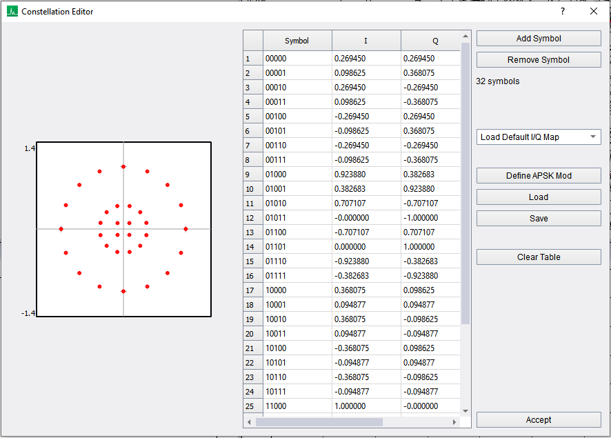
APSK32 in the constellation editor.
APSK Editor
Opened via the Define APSK Mod button in the Constellation Editor. Four parameters define each APSK ring, editable in the table:
- Ring ID – ID number where 0 is the innermost ring.
- **# States** – Number of symbols represented in this ring.
- R#/R0 – Ratio of this ring's radius to the innermost ring (R0).
- Phase – Phase offset of the first state in this ring.
Additional controls:
- Load Default I/Q Map – Populates the constellation table with a default selection.
- Add Row – Adds another ring to the table.
- Remove Row – Removes the last ring from the table.
- Load – Load a previously saved APSK configuration.
- Save – Save the current configuration to a CSV file.
- Accept – Validates that the total number of states is a power of 2, stores the data, and closes the window.
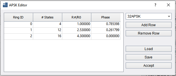
APSK32 in the APSK editor.
Wide Carrier Estimation
When enabled, wide carrier estimation performs an additional search step over a custom frequency range, allowing demodulation of signals with large carrier frequency error. This step sweeps the user-specified range prior to demodulation, performs an occupied bandwidth measurement, and uses the center of the estimated occupied bandwidth as the new demodulation center frequency. This step is performed before each demodulation measurement.
The range should be set to at least twice the maximum expected frequency error plus half the signal bandwidth:
Range = 2 × (CF_error + BW/2)
Sync Search
When sync search is enabled, demodulation occurs over a window of Search Length symbols. The sync pattern is searched for within this window. If found, the position of the first matching symbol is used to frame the measurement, with an additional optional offset applied.
- Search length must be longer than the measurement length. The measurement cannot extend beyond the search length.
- If the offset adjusts the result window outside the search window, the pattern is considered not found.
- Sync search can be combined with triggering. When used on pulsed waveforms, ensure the search length does not exceed the pulse duration.
- If the sync pattern appears more than once in the search window, only the first occurrence is used.
- If the pattern is not found, "Pattern Not Found" is displayed on the demod bits plot.
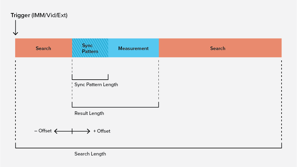
This diagram illustrates how sync search is performed and how the measurement is framed within the search length.
Equalization
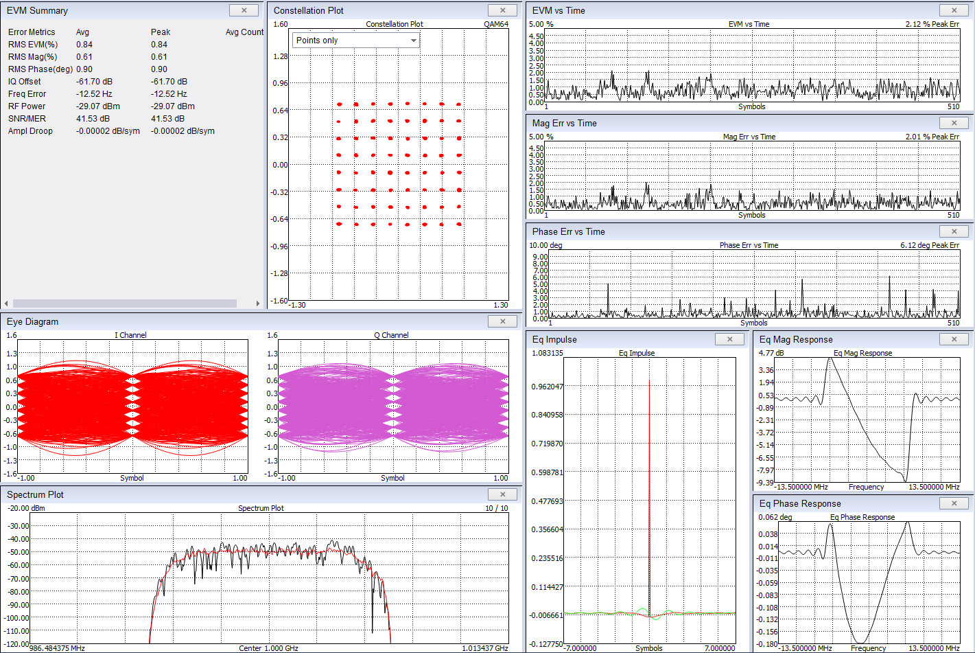
Characterizing a QAM64 waveform over a heavily impaired channel using equalization.
Equalization measures and corrects for amplitude and phase frequency response (group delay) across the measurement channel due to fading, multipath, reflections, or system components such as filters and amplifiers. This isolates non-linear errors by removing linear impairments.
Equalization is only available for PSK and QAM modulation formats.
Spike uses a complex adaptive LMS FIR filter. Adaptation is performed on the measured and reference waveforms, and the resulting filter weights are applied to the I/Q data on the next measurement, prior to symbol lock, carrier recovery, and demodulation.
Since equalization is performed blind (no training sequence), large EVM and bit errors may hinder convergence. Ensure the signal's frequency error is a small percentage of the symbol rate — 1% or less is recommended. Tune the analyzer to an ideal center frequency before running equalization.
The equalization filter resets under these conditions:
- Program startup
- Leaving and re-entering digital demodulation mode
- Measurement filter change
- Symbol rate change
- Equalizer filter length change
- The Reset Filter button is pressed
Tap count formula: Tap count = (User Selected Filter Length − 1) × Pts/Sym + 1
The user-selected convergence factor is scaled internally by 1.0×10⁻⁶. Larger values adapt faster but are more susceptible to noise and instability. Smaller values adapt more slowly but resist noise. Starting values between 1–100 are recommended for quick convergence, then reduce as EVM improves.
If the filter becomes unstable, it is no longer applied and waits for a manual reset — instability is visible on the equalization plots. The filter impulse response, frequency response, and phase response can be viewed in the equalizer plots. The impulse response can be exported via the context menu.
High Order QAM Signals
Tips for measurements with high-order QAM modulations:
- Set measurement length to 2–4 times the modulation order (e.g., 512–1024 symbols for 256QAM).
- Ensure adequate symbol randomness — ideally all constellation points are hit within a single measurement.
- Keep frequency error small; even small errors cause invalid results. Use lower-order modulations to measure and compensate for frequency offset beforehand, or use a common timebase.
- Measurements can take several seconds to over a minute for large, high-order captures. The measurement must complete before configuration changes are accepted — verify all settings before selecting the high-order QAM modulation.
Measurement Plots
Measurement displays can be added to the main view area using the Add View combo box on the toolbar. With Auto Fit enabled, views are arranged in an organized grid. With Auto Fit disabled, views can be freely moved and resized. The layout is saved on close and restored on the next launch.
All plots in digital demodulation mode follow the Basic Plot interface in Spike.
Error Summary
Displays modulation quality metrics including EVM, phase error, magnitude error, and frequency error. Most values are provided as peak and RMS averages over a user-selected sample size. Error values are first averaged per symbol over the capture interval, then peak-held and RMS-averaged for display. For per-symbol error over a single capture, see the Error vs Time plots.
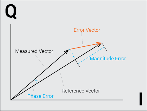
Visualization of the EVM, magnitude, and phase error calculations.
Metric definitions:
EVM – Root mean square of the error vectors, normalized to the maximum constellation magnitude, expressed as a percentage.
\( \large EVM(\%) = \frac{\sqrt{\frac{1}{N} \sum_0^{n-1}{(I_{error}^2 + Q_{error}^2)}}}{\text{Normalization Reference}} * 100% \)
Magnitude Error – Per-symbol difference between reference and measured magnitudes, normalized to the maximum constellation magnitude. RMS and peak are calculated across all symbols in the capture window.
\( \large Magnitude_{Err}[n] = \frac{|Mag_{Ref}[n]| - |Mag_{Meas}[n] |} {\text{Normalization Reference}} \)
Phase Error – Per-symbol difference between reference and measured angle.
\( \large Phase_{Err}[n] = Angle_{Reference}[n] - Angle_{Meas}[n] \)
FSK Error – is defined as,
\( \large FSK_{Err} = \frac{RMS(FSK_{Err} \text{at Each Symbol})}{Deviation} \)
Where the FSK error at each symbol is
\( \large FSK_{Err} \text{at Symbol i} = FSK_{Meas}[i] - FSK_{Ref}[i] \)
- Frequency Error – Difference between the user-supplied center frequency (reference) and the measured carrier frequency.
The normalization reference is 1.0, defined as the maximum constellation magnitude. Spike forces the largest constellation magnitude to equal 1 for all selectable modulations.
Constellation Diagram
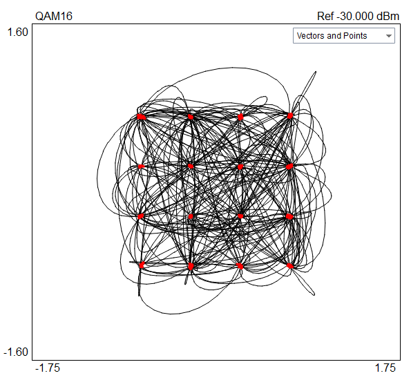
Constellation diagram for a QAM16 signal.
Displays the modulation states and transitions of the input signal on the complex plane, helping visualize signal quality and identify impairments such as phase noise, amplitude imbalance, and quadrature error.
Symbol Table
Displays the demodulated bits of the input signal. The number of bits shown equals the symbol count times the bits per symbol for the selected modulation type. Bits can be displayed in binary or hexadecimal format. The trigger pattern and whether it was detected are also shown.
Eye Diagram
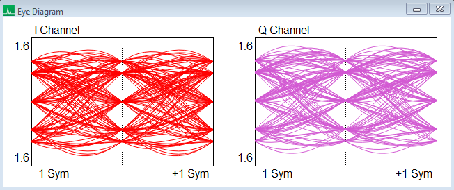
Eye diagram for a Pi/4DQPSK signal.
Visualizes system performance characteristics such as signal distortion, inter-symbol interference, signal-to-noise ratio, and timing errors.
Error vs Time
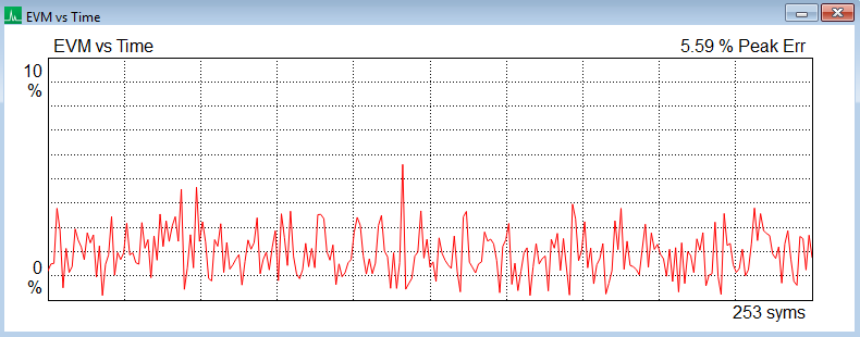
EVM vs time plot.
Provides symbol-resolution views of common quality metrics (EVM, magnitude error, phase error) for each symbol in the configured capture.
EMC Precompliance
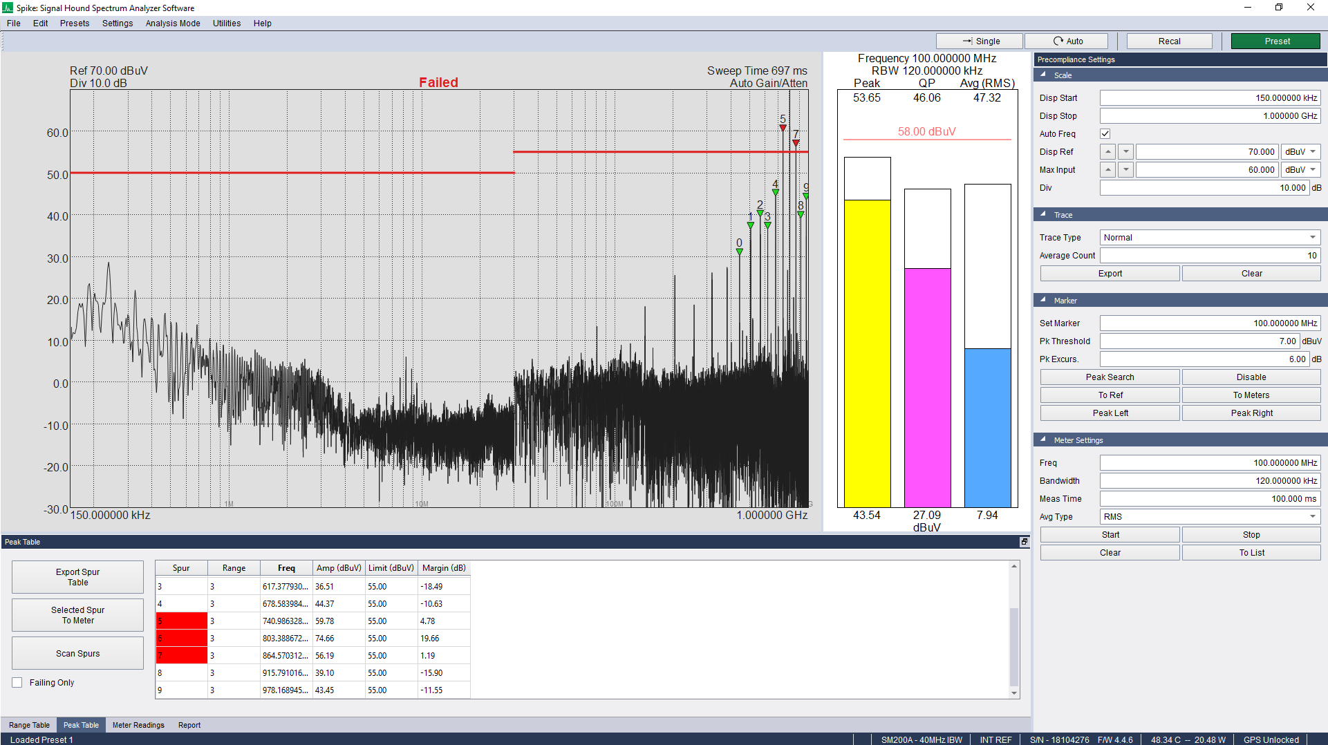
Radiated emissions testing on a noisy synthesizer.
Precompliance measurements are available for SM, SP, and BB series devices, accessed via Analysis Mode > EMC Precompliance. This mode provides measurement functions for testing emission regulation requirements, including:
- Up to 10 log-scaled sweep ranges with custom limits and sweep parameters.
- Path loss and antenna factor tables for calibrating the test setup.
- A spur table listing all signals that exceed user-defined limits and thresholds.
- Quasi-peak, peak, and average detectors for signals of interest, shown in the bar meter plot.
- Detector lists that store bar meter results.
Pre-Compliance Control Panel
- Disp Start / Disp Stop – Start and stop frequencies for the trace display when Auto Freq is disabled.
- Auto Freq – When enabled, the trace display spans the full frequency range of all active EMI sweeps. When disabled, the display spans only the Disp Start/Stop range, useful for viewing a specific region of interest.
- Disp Ref – Reference level for the trace display.
- Ref Level – Specify the maximum expected input signal level. Controls receiver sensitivity and applies to all active sweep ranges. Set approximately 5 dB above the largest expected input.
- Div – Adjust the y-axis scale of the plot.
- Trace Type – Select between clear-and-write, max-hold, and average trace behavior. All ranges follow this setting.
- Average Count – Number of trace averages when trace type is Average. Applies to all ranges.
- Export – Export the current sweep to a CSV file.
- Clear – Clear the displayed sweep.
- Set Marker – Manually set the marker frequency.
- Pk Threshold – Minimum amplitude for a signal to be considered a peak for the peak left/right buttons.
- Pk Excurs. – How far the amplitude must fall around a peak for it to qualify as a peak for the peak left/right buttons.
- Peak Search – Set the marker to the frequency of the largest amplitude signal.
- Disable – Hide the displayed marker.
- To Ref – Set the reference level to the current marker amplitude.
- To Meters – Set the bar meter frequency to the current marker frequency.
- Peak Left / Peak Right – Move the marker to the next peak to the left or right.
- Freq – Select the meter center frequency.
- Bandwidth – Select the bandwidth used for meter readings.
- Meas Time – Select the acquisition time for meter readings.
- Start / Stop – Start or stop meter detection. While detector measurements are active, sweeps pause.
- Clear – Clear the current and peak meter readings.
- To List – Store the current meter readings to the meter list.
Range Table
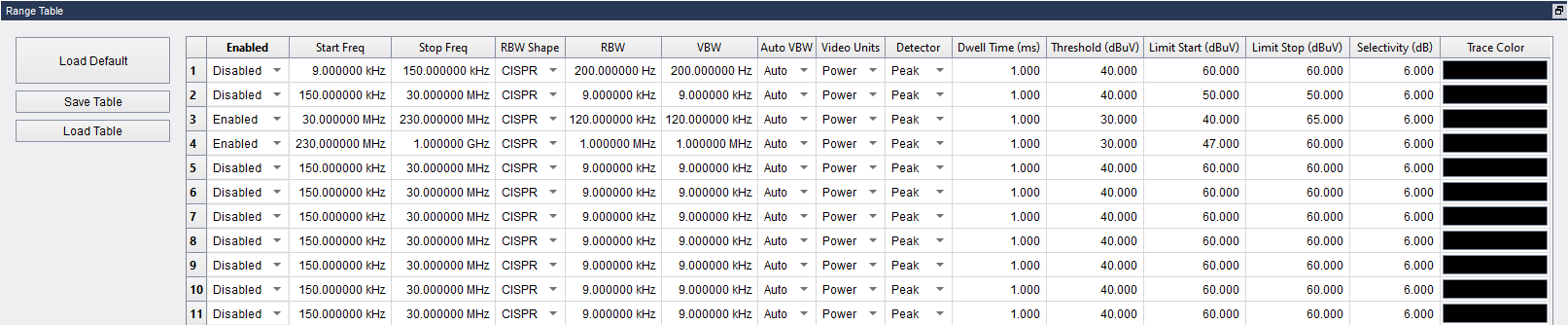
Range table controls.
The range table allows customization of up to ten sweep ranges, each with its own frequency range, RBW, VBW, and test limits. Changes take effect immediately and the table can be saved and reloaded.
- Load Default – Load the default range table inputs.
- Save Table / Load Table – Save or load the table setup as a CSV file.
- Enabled – Enable or disable the selected range. Enabled ranges are swept and shown on the frequency scan display.
- Start Freq / Stop Freq – Frequency bounds of the selected range.
- RBW Shape – Select between the 6 dB CISPR RBW (Gaussian) or Flat-Top 3 dB RBW filter.
- RBW – Resolution bandwidth.
- VBW – Video bandwidth.
- Auto VBW – When enabled, VBW tracks RBW. When disabled, VBW must be ≤ RBW.
- Video Units – Video processing unit type.
- Detector – Select between Peak and Average detectors.
- Dwell Time – Duration the spectrum analyzer dwells at each frequency. Useful for capturing periodic events. Recommended to use with the peak detector when increasing dwell time.
- Threshold – Minimum signal level for a signal to be considered a spur. Must be lower than the limit setting.
- Limit Start / Limit Stop – Amplitude limits at the start and stop frequency of the range. A flat limit is achieved by setting both values equal. The limit line is interpolated on a logarithmic frequency scale.
- Selectivity – Determines spur detector sensitivity. Higher values require greater separation for a signal to be flagged as a spur. Low values may greatly increase the number of reported spurs.
Frequency Scan Display
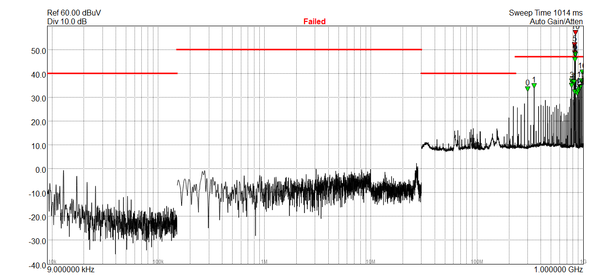
Frequency scan display showing 4 configured sweep ranges.
The main display for precompliance measurements. Shows all configured sweep ranges on a single logarithmically-scaled frequency axis, spanning the minimum to maximum configured frequencies. Red limit lines and numbered spur markers are overlaid on the trace. A single marker is available by clicking anywhere on the spectrum.
The trace can be configured as max-hold or normal. Max-hold is useful for capturing intermittent or short-duration signals.
Spur Table
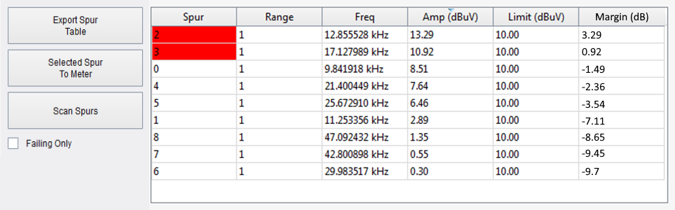
Spur table sorted by spur amplitude.
Lists all signals above the minimum threshold set for each sweep range. Spur numbers correlate to the numbered markers on the frequency scan display. Up to 100 spurs are shown. Spurs that exceed the range limits are highlighted red.
To measure spurs of interest: press Single to pause sweeping (freezing the spur table), then sort by frequency or amplitude and use Selected Spur to Meter to route a spur to the bar meter.
- Export Spur Table – Export the peak table and meter list to a CSV file.
- Selected Spur to Meter – Move the selected spur frequency to the meter frequency input.
- Scan Spurs – Take meter measurements at all spurs and add results to the Meter Readings list.
- Failing Only – When using Scan Spurs, measure only spurs that exceed the limit.
- Spur – Spur number, ordered by frequency by default.
- Range – The configured range in which the spur falls.
- Freq – Frequency of the spur.
- Amp – Amplitude of the spur.
- Limit – Interpolated limit at the spur frequency.
- Margin – Difference between amplitude and limit (Amp − Limit).
Bar Meters
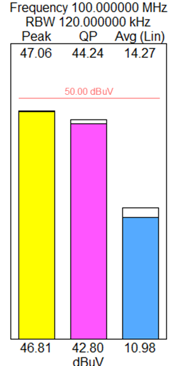
Bar meters measuring a pulsed signal.
The bar meters display shows three detector readouts at a single center frequency and is the second measurement tool for precompliance testing. Start and stop meter detection using the Start and Stop buttons on the control panel — sweeps pause while detector measurements are active. Detection also starts automatically when Selected Spur to Meter is clicked.
The bar meters show up to four detectors: peak and quasi-peak are always shown; the average detector can be set to RMS or linear average. A red limit line is shown at the meter frequency, interpolated from the Range Table limits.
Meters update at the rate set by Meas Time. Max-held detector values are stored since the last Clear. Press To List to save current peak detector values to the meter list.
Meter List

Meter readings results.
Generated by taking detector measurements at various frequencies and saving them with To List, or by clicking Scan All in the spur table panel. The list can be exported to a CSV file.
- Export Meter Readings – Export all meter readings to a CSV file.
- Delete Selected – Remove the selected meter reading(s).
- Clear List – Remove all readings from the list.
- Frequency – Frequency at which the meter reading was taken.
- RBW – Resolution bandwidth of the measurement.
- Peak / Quasi Pk / Avg – Detector results of the measurement.
- Limit – Interpolated limit at the measurement frequency.
- Date/Time – Timestamp of the reading.
- Comments – Entry field for notes about the reading.
Report Panel

PDF report configuration and generation.
The report panel generates a formal PDF report of precompliance test results. The report includes all Meter Readings in tabular form, a snapshot of the sweep plot, entered metadata, and a full description of the spectrum analyzer used (manufacturer, model, serial number, firmware version).
- Generate Report – Generate and save the PDF report to a chosen location.
- Clear Info – Clear all metadata entry fields.
- Report Number – Identifying number for the report.
- DUT Name – Name of the product under test.
- DUT Info – Additional description of the product under test (e.g., serial number).
- Date of Test – Date the readings were carried out.
- Test Engineer – Engineer responsible for the test.
- Notes – Additional information.
Quasi-Peak Measurements
Quasi-peak (QP) measurements are available through the bar meters display and begin when pressing Start on the precompliance settings control panel. The QP detector in Spike conforms to the CISPR 16.1 and ANSI C63.2 standards.
| Frequency Range | Charge Time Constant | Discharge Time Constant |
| 9 – 150 kHz | 45 ms | 500 ms |
| 150 kHz – 30 MHz | 1 ms | 160 ms |
| 30 MHz – 1 GHz | 1 ms | 550 ms |
The charge time constant is the time required, after instantaneous application of a constant RF sine wave, for the output to reach 63% of its final value. The discharge time constant is the time for the output to fall to 37% of its initial value after the signal is removed.
Damped Output: The QP detector output is simulated as a critically damped meter with a time constant of 160 ms for 9 kHz – 30 MHz and 550 ms for 30 MHz – 1 GHz. Both the detector and damped output are realized in Spike using digital filters.
Analog Demodulation
Analog demodulation performs modulation quality measurements on AM and FM signals. Analysis can be performed on signals with an AM and FM modulation rate of up to 20kHz, and total occupied bandwidth of 200kHz (+/- 100kHz deviation).
Analog Demodulation Measurements
Basic measurements performed on the audio signal,
- Carrier Frequency – Records the carrier frequency.
- Carrier Error – Difference between the measured carrier frequency and the configured center frequency.
- Avg Power – Average power of the entire capture in dBm.
- Peak (+/−) – Minimum and maximum peak of the audio signal (Hz for FM, depth% for AM).
- RMS – Root mean square of modulation (Hz for FM, depth% for AM).
- Modulation Rate – Frequency of the AM/FM modulation.
- SINAD – Signal-to-Noise and Distortion ratio. See equation below.
- THD – Total Harmonic Distortion: The RMS of the first nine harmonics relative to the fundamental. See equation below.
Both SINAD and THD measurements apply to the demodulation type selected for Zero-Span (AM or FM).
\( {\large SINAD = \frac{P_{signal} + P_{noise} + P_{distortion}}{P_{noise} + P_{distortion}} } \)
\( { \large THD = \frac{\sqrt{V_2^2 + V_3^2 + ⋯ + V_9^2}} {V_1} } \)
Analog Demodulation Plots
The results are displayed on the following plots.
- AM Time Domain – Shows amplitude modulation over time, shown in the units specified by the Input Level settings.
- AM Spectrum – Displays the frequency spectrum of the AM waveform. The y-axis shows AM depth% on a logarithmic scale using 100% depth as the reference.
- FM Time Domain – Shows the FM demodulated signal vs time.
- FM Spectrum – Displays the frequency spectrum of the FM waveform. The y-axis is frequency deviation in Hz, with the reference level equal to the device sample rate.
- Analysis Summary – Displays modulation measurement results for AM and FM waveforms.
Analog Demodulation Control Panel
Configure measurements by selecting the input signal power level, carrier frequency, and low-pass filter in the right-hand control panel. The low-pass filter is applied to the demodulated signal before modulation analysis. Changes take effect immediately.
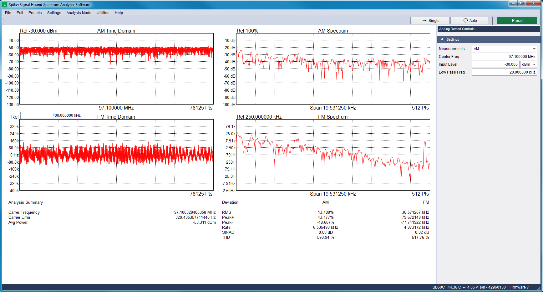
Viewing a broadcast FM signal and observing the 19kHz FM pilot tone.
Interference Hunting
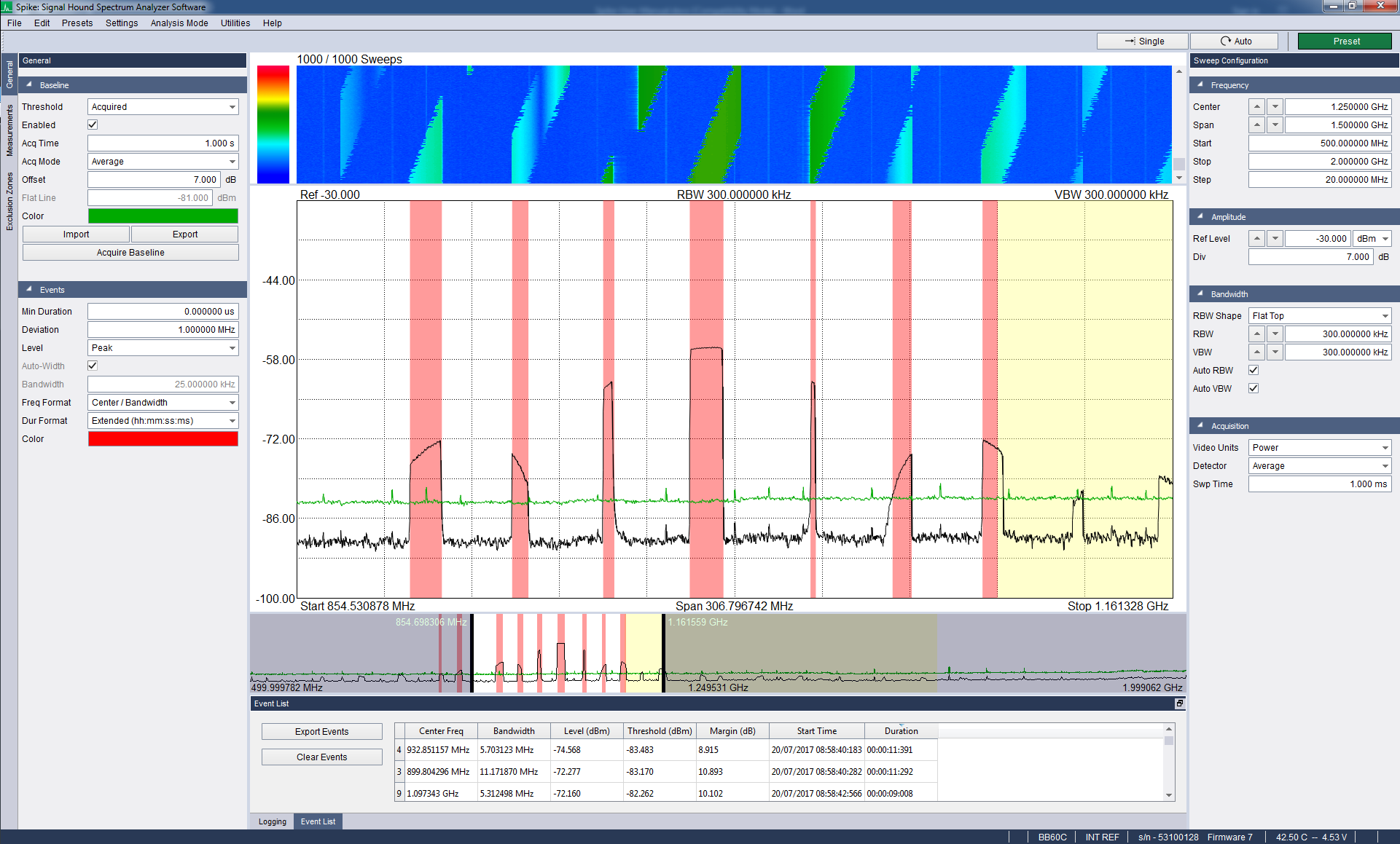
Detecting events exceeding a defined baseline with exclusion zones.
Interference Hunting mode provides tools to spot and characterize interfering RF signals. An elevated noise floor on a receive channel indicates likely interference. The interfering signal may not be on the channel itself, but must be within the analyzer's bandwidth.
A signal is detected by setting a baseline — an amplitude threshold above which a signal is considered suspicious. Any time a signal exceeds the baseline, an event is created containing: frequency, bandwidth, peak level or channel power, threshold, margin (dB over threshold), start time, and duration.
Events appear in an on-screen list updated after every sweep and can be logged to a CSV file as they occur. Logging enables unmanned operation over extended periods, automatically capturing all relevant details of intermittent signals for later inspection.
Setting a Baseline
A baseline can be a flat line (single amplitude threshold) or an acquired baseline built from sweeps over a period of time (e.g., a max-held noise floor image). A flat baseline is set instantly by choosing a threshold level. An acquired baseline requires setting an acquisition time interval and mode (min hold, max hold, or average). After acquisition, a dB offset can be applied. Acquired baselines can be exported and imported in CSV format.
A flat baseline.
An acquired baseline.
Baseline File Format
A baseline CSV file consists of a header and a list of (frequency, amplitude) pairs:
BASELINE, Version 1
startFreq, 2.00E+09
binSize, 100.0E+06
RBW, 30.0E+03
VBW, 30.0E+03
refLevel, -20.00
div, 10.00
timestamp, 1.50714E+12
offset, 5.00
frequency(Hz), amplitude(dBm)
2.00E+09, -50.00
2.10E+09, -51.00
...
The frequency of each point is inferred from startFreq and binSize — listed frequencies are for reference only and are not used on import. RBW, VBW, refLevel, div, and timestamp are also reference-only. offset is the dB offset set in the General Control Panel. Custom baseline files can be created or edited in a spreadsheet and imported.
Defining Events

A single-sweep snapshot of an event.
An event is the portion of a signal that exceeds the baseline within a single sweep. Because events have a time dimension across multiple sweeps, two parameters govern what constitutes a continuous multi-sweep event:
- Deviation – Maximum allowable center frequency difference between consecutive snapshots for them to be considered the same event.
- Minimum Duration – Minimum time a signal must persist before being logged as an event.
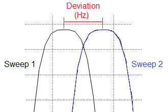
The frequency deviation between two single sweep snapshots of an event.
To catch quick or frequency-jumping signals: set minimum duration to zero and deviation to a high value. For persistent, steady signals: increase minimum duration and lower deviation.
Regional Zoom

Regional zoom view.
Regional zoom allows close visual inspection of a specific portion of the spectrum without changing the sweep span. The regional zoom controller appears as a horizontal strip below the main sweep plot. Drag the left and right bounds (vertical black lines) to adjust the visible region, or drag the entire unshaded window. The full sweep, including baselines and events, is always visible in the controller.
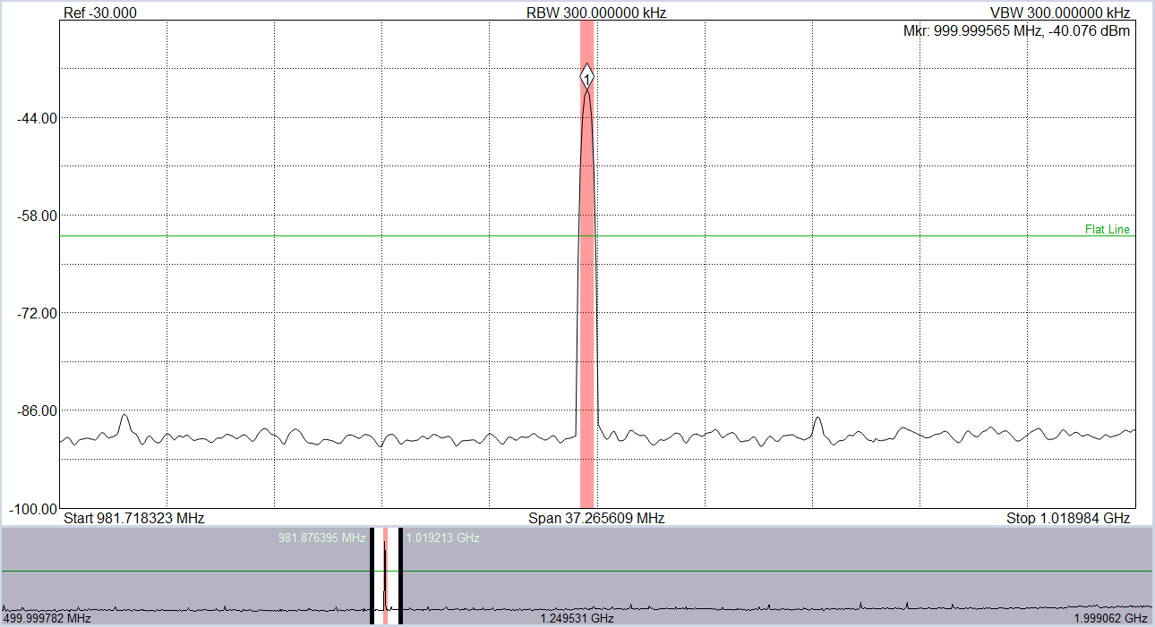
Regional zoom used for close up inspection of an event.
Exclusion Zones
Exclusion zones are frequency ranges where events cannot occur, used to ignore known signal sources and reduce false positives. A zone is defined by a start and stop frequency. Signals within an exclusion zone are not flagged as events even if they exceed the baseline.
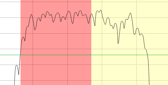
A signal breaking a flat baseline and falling partially within an exclusion zone. Only the unexcluded part of the signal is considered an event (red shaded portion).
Spectrogram
The spectrogram (waterfall) can optionally appear above the main plot. See Spectrogram for more detail.
Sweep Settings Control Panel
See Sweep Settings Control Panel in Swept Analysis mode.
Interference Hunting Toolbar
- Spectrogram – Enables the spectrogram display.
General Control Panel
Divided into two sections: Baseline and Events.
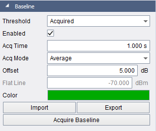
Baseline control panel.
Baseline
- Threshold – Specifies the baseline type: acquired or flat line.
- Enabled – Specifies whether the baseline is displayed on plots and used for event detection.
- Acq Time – Duration over which a new baseline is acquired.
- Acq Mode – Accumulation function applied to consecutive sweeps during acquisition (min hold, max hold, or average).
- Offset – Amplitude offset applied to the acquired baseline from its original level.
- Flat Line – The constant amplitude threshold used when a flat baseline is selected.
- Import / Export – Load or save a baseline file.
- Acquire Baseline – Begin acquiring a new baseline using the current acquisition settings.
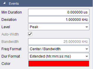
Events control panel.
Events
- Min Duration – Minimum time a signal must exceed the baseline to be considered an event.
- Deviation – Allowable center frequency variation for an event across sweeps.
- Level – Mode of level calculation: Peak (highest amplitude) or Channel Power (channel power at the event center frequency).
- Auto-Width – In Channel Power mode, automatically selects a bandwidth for channel power computation.
- Bandwidth – In Channel Power mode, manually specify the bandwidth for channel power computation.
- Freq Format – Frequency format used in the event list and logging: Center/Bandwidth or Start/Stop.
- Dur Format – Duration format: Basic (s) for seconds, or Extended (hh:mm:ss:ms) for clock format.
- Color – Color of events displayed on the plots.
Measurements Control Panel
See Measurements Control Panel in Swept Analysis mode.
Exclusion Zones Control Panel
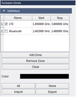
Exclusion zone control panel.
- Add Zone – Adds a new exclusion zone to the list and activates it.
- Remove Zone – Removes the highlighted exclusion zone from the list.
- Clear – Removes all exclusion zone definitions.
- All / None – Activates or deactivates all exclusion zones in the list.
- Import / Export – Import or export the exclusion zone list.
Logging Control Panel

Logging control panel.
Events are logged in real time to a CSV file. Logging continues until manually cancelled, a set time elapses, or a maximum event count is reached.
- Save Directory – Default directory for CSV event log files.
- File Prefix – Prefix applied to all saved file names.
- Capture Size – Length of time during which logging takes place.
- Unlimited Events – No upper limit on captured events; logging continues for the full capture duration.
- Max Events – Maximum number of events that can be logged in one capture.
- Max File Size – Maximum file size for a CSV log file.
Event List

Event list.
The event list updates after every sweep. It can be sorted by any column and exported to CSV. When events are cleared, all future events are treated as new, with start times and durations reset.
- Export Events – Save the current event list to a CSV file, preserving the current sort order.
- Clear Events – Delete all events from the event list.
Spectrum Emission Mask
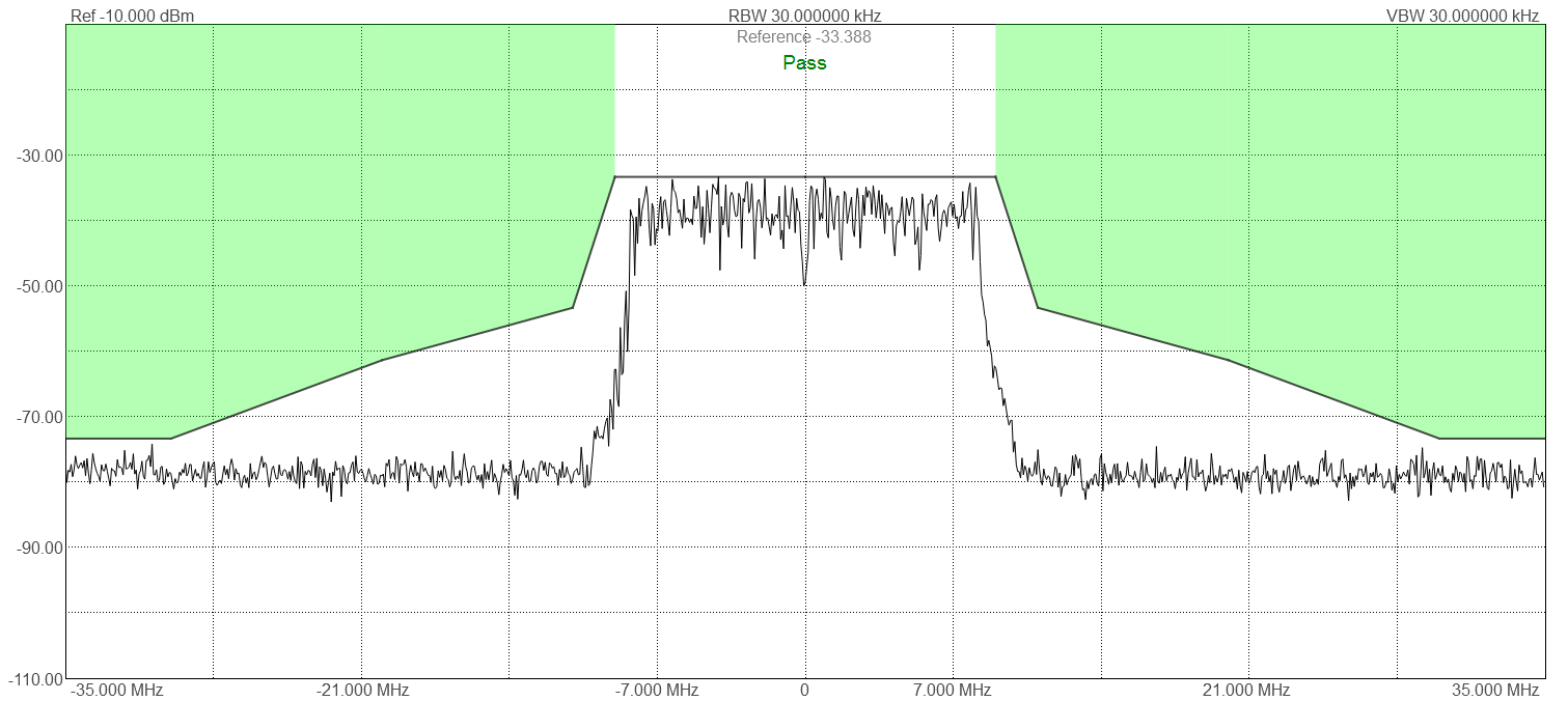
Testing input against an 802.11 OFDM transmission mask.
The Spectrum Emission Mask (SEM) measurement detects out-of-band spurious, interfering, and excessive emissions. Emissions are tested against a user-defined mask specified as amplitude offsets relative to the in-band signal power at frequency offsets from the center frequency.
Masks are entered manually in the offset table, or loaded from preset masks built into Spike. Mask offsets are drawn on the graticule as shaded regions — green for passing, red for failing.
Set the input level as close to the expected input power as possible to maximize dynamic range. An IF overload message appears if the input power is set too low.
All offsets are measured relative to an amplitude reference, determined by a peak measurement, channel power, or direct user entry. The reference span defaults to the range between the first configured offset and is recalculated each sweep.
Control Panel
- Center Freq – Reference frequency for the offset table and tuned center frequency of the sweep.
- Step – Frequency step size for the center frequency arrows.
- Span – Frequency span around the center frequency.
- RBW – Resolution bandwidth, using a flat-top window.
- VBW – Video bandwidth.
- Ref Level – Maximum expected input level of the signal.
- Div – Controls the plot y-axis scale.
- Video Units – Unprocessed amplitude data representation: voltage, linear power, or logarithmic power. Linear power is used for RMS measurements; logarithmic is closest to a traditional spectrum analyzer.
- Detector – Choose whether min/max or average amplitudes are stored during video processing.
- Trace Type – Select clear/write or max-hold trace behavior.
- Meas Type – Specify how the reference amplitude is measured.
- Reference – Directly specify the amplitude reference.
- Width Set – Specify the frequency range over which the channel power amplitude reference is calculated. When set to Auto, the span between the center frequency and the first offset is used. When set to Manual, the entered width is used.
- Width – Direct-set width value.
- Meas Width – Actual measurement width (read-only).
- Load Mask – Load a predefined offset table.
Context Menu
- Show Pass/Fail Indicator – Toggles visibility of the pass/fail indicator at the top center of the graticule.
Configuring Offsets

Spectrum emission mask offset table editor.
Up to 16 offsets can be configured. Each offset can be tested against an absolute amplitude or one relative to the measured in-band channel power, and can have a linear shape (flat or sloped). Offsets are configured as upper offsets but are applied symmetrically as both upper and lower offsets around the center frequency.
Results

Spectrum emission mask results table.
The results table shows the largest margin for both the upper and lower offset on each row. The frequency and level columns display the frequency and amplitude of the worst-case margin in each offset. Results can be exported to a CSV file.
Limitations
Not all Signal Hound devices support all spectrum emission mask measurements. The dynamic range limitations of some devices (SA44, SA124, BB60 series) may prohibit certain mask measurements such as AM/FM masks at outer offsets. Disabling outer offsets may be necessary to avoid failing measurements on these devices.
The legacy Signal Hound software performed custom sweeps to overcome dynamic range limitations of SA series devices. These custom sweeps are not performed in Spike, and results may differ from the legacy software — particularly for FM broadcast mask measurements.
Noise Figure
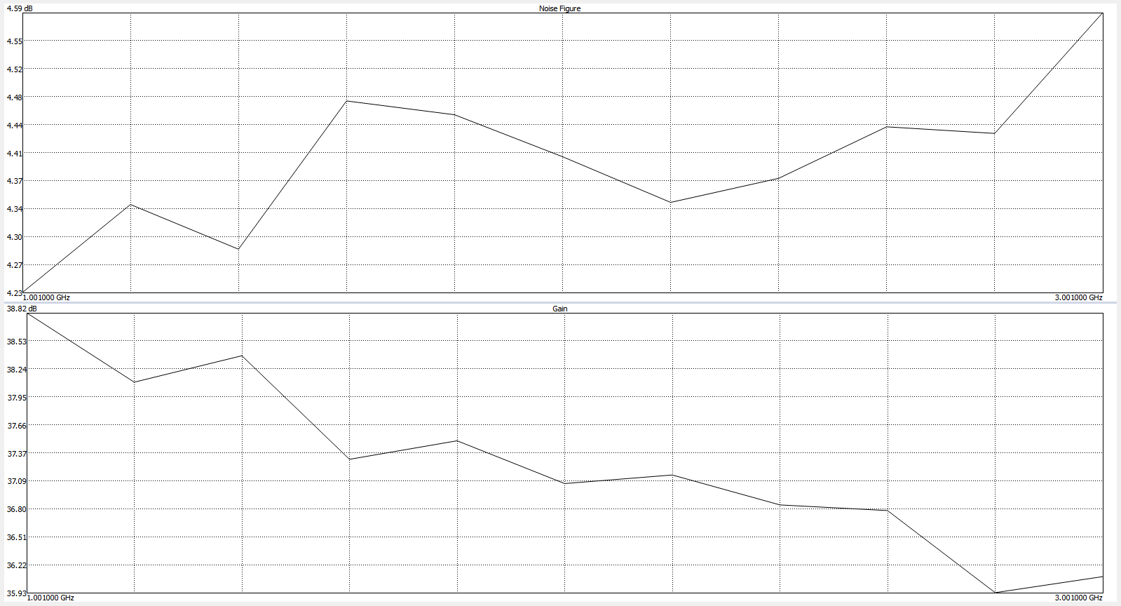
Noise figure and gain plots of a small wideband amplifier.
Noise figure measurements are available for SM, SP, and BB series devices.
Noise figure is a measure of the noise a device contributes to a signal, expressed as the degradation in signal-to-noise ratio as the signal passes through the device. It is computed using the Y-factor technique from several spectrum analyzer measurements.
Process Overview
The measurement consists of two steps, each measuring noise power with the noise source in ON and OFF states:
- Calibration – Noise source connected directly to the spectrum analyzer.
- DUT Measurement – DUT inserted between the noise source and the spectrum analyzer.
DUT properties are derived from the difference between the two steps. Once calibrated for the current configuration, repeated measurements can be taken without recalibrating.
The Y Factor Method
The Y factor technique is a common method of calculating noise figure (NF). Its computations are carried out in terms of noise temperature (T) in linear scale.
Noise figure is expressed on the logarithmic scale. Noise factor (F) is the linear equivalent,
\( NF = 10 * log_{10}(F) \)
The Y factor is defined as the linear ratio of noise power level when the noise source is ON and OFF,
\( Y = \frac{N_{ON}}{N_{OFF}} \)
The Y factor can be converted to noise temperature,
\( T = \frac{T_{SourceON} - Y(T_{SourceOFF})} {Y-1} \)
where 𝑇_𝑆𝑜𝑢𝑟𝑐𝑒𝑂𝑁 is the excess noise ratio (ENR) of the noise source, and 𝑇_𝑆𝑜𝑢𝑟𝑐𝑒𝑂𝐹𝐹 is the ambient room temperature, generally considered to be 290 K.
Noise factor can then be derived from noise temperature,
\( F = 1 + \frac{T}{T_{SourceOFF}} \)
The measurement setup is considered a two-stage system, where the DUT is stage 1, and the spectrum analyzer is stage 2. The noise factor of a two-stage system (F12) can be derived from the noise factors of its component stages (F1, F2) and the gain of its first stage (G1),
\( F_{12} = F_1 + \frac{F_2 - 1}{G_1} \)
This equation can be written in terms of noise temperature for stage 1,
\( T_1 = T_{12} - \frac{T_2}{G_1} \)
DUT Gain is computed,
\( G_1 = \frac{N^{ON}_{12} - N^{OFF}_{12}}{N^{ON}_2 - N^{OFF}_{12}} \)
Control Panel
- Freq Mode – Choose between Swept and Fixed mode. In swept mode, measurement points are distributed evenly across the span. In fixed mode, only the Fixed Freq is tested.
- Start/Stop – Lowest and highest test frequencies (non-fixed mode).
- Center – Center of the test frequency range (non-fixed mode).
- Span – Range of test frequencies (non-fixed mode).
- Points – Number of evenly spaced test frequencies across the span (non-fixed mode).
- Fixed Freq – Frequency tested in fixed mode.
- Ref Level – Power level of the top graticule line.
- RBW – Resolution bandwidth, using a flat-top window.
- VBW – Video bandwidth.
- Auto RBW / Auto VBW – Automatically select RBW (and set VBW = RBW) relative to the measurement span. Recommended when changing span.
- Meas Span – Span of sweeps taken during measurement at each test frequency.
- Averaging – When enabled, averages the specified number of power readings at each test frequency.
- Avg Number – Number of sweeps averaged at each test frequency when averaging is enabled.
- Room Temp – Ambient room temperature in Kelvin.
- Play Alert – When enabled, a sequence of beeps plays when a full sweep through all measurement points completes.
- Noise Source (Cal) – Select the noise source for the calibration step.
- Noise Source (Meas) – Select the noise source for the measurement step.
- Manage ENR Tables – Opens the ENR table manager.
Noise Sources & ENR Tables
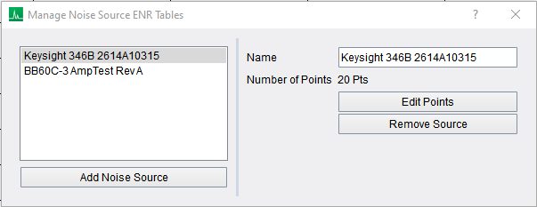
Noise source ENR table manager.
When the noise source is ON, its "hot" noise temperature is the Excess Noise Ratio (ENR) at the frequency being measured. The ENR table — usually printed on the noise source — must be entered manually for accurate measurements.
The ENR Table Manager allows adding, removing, renaming, and editing ENR table entries. It is accessed via Manage ENR Tables. Tables persist across sessions until deleted and are saved/loaded with global presets, matched by name to the current noise source list.
Results Table

Noise figure results table.
Displays the measured noise figure and gain at each tested frequency. Exportable as a CSV file via Export Results Table.
Making Measurements
Noise figure measurements follow a manual step-by-step process. A measurement can be cancelled at any time with the Abort button, reverting state to before the measurement began.
Calibration (Optional)
Calibration establishes a baseline accounting for the analyzer's noise contribution (second-stage correction). It can be skipped if the DUT has high gain (>30 dB) and the analyzer has low noise figure; otherwise, skipping typically results in substantially higher errors. Calibration is required for gain measurement.
Calibration is initiated with the Calibrate button on the main toolbar. Calibration data is stored in memory for the Spike session, or until the configured measurement points change. If other settings (sweep, averaging) change, the calibration remains valid but at reduced accuracy.
Calibration states shown in the toolbar:
- Uncal (red) – No valid calibration stored. High measurement error is likely unless the DUT has ≥30 dB gain.
- Cal (yellow) – Valid calibration stored, but accuracy is reduced due to configuration changes since the last cal.
- Cal (green) – Valid calibration whose settings match the current configuration exactly.
Measurement Process
- Configure the measurement: define the frequency list, sweep settings, averaging, room temperature, and ENR table.
- (Optional) Calibrate: connect the noise source directly to the analyzer and follow prompts to toggle the noise source ON and OFF.
- DUT measurement: insert the DUT between the noise source and the analyzer and follow prompts to toggle the noise source OFF and ON.
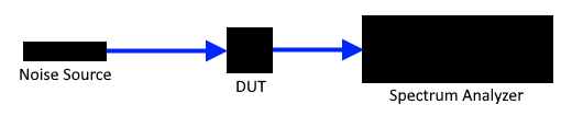
Noise figure DUT measurement step setup.
- View results in the Noise Figure and Gain plots and the Results table. Repeat steps 2–3 as desired, or return to step 1 for a new configuration.
Annunciator List
Invalid – Noise figure or gain calculation failed. Occurs when the ON-state signal is not higher than the OFF-state signal. Remedies: use a noise source with higher ENR, increase averaging, increase meas span, or lower the reference level for maximum sensitivity.
Recommended reference levels for maximum sensitivity:
| Device | Reference Level |
| SM200/435 | −20 dBm or lower |
| SP145 | −30 dBm or lower |
| BB60C | −50 dBm or lower |
| BB60D | −30 dBm or lower |
- IF Overload – An IF overload occurred during a measurement. See "IF overload" in Annunciator List.
- IF Overload (Cal) – An IF overload occurred during the calibration used by the measurement. See "IF overload" in Annunciator List
Limitations
- SA Series – Noise figure measurements are not available. Software image rejection makes SA series devices unsuitable for broadband noise signals.
- BB Series – For best results, keep ENR + gain below 40 dB.
- SP Series – For best results, keep ENR + gain below 50 dB.
- SM Series – For best results, keep ENR + gain below 60 dB.
SUN-OFDM
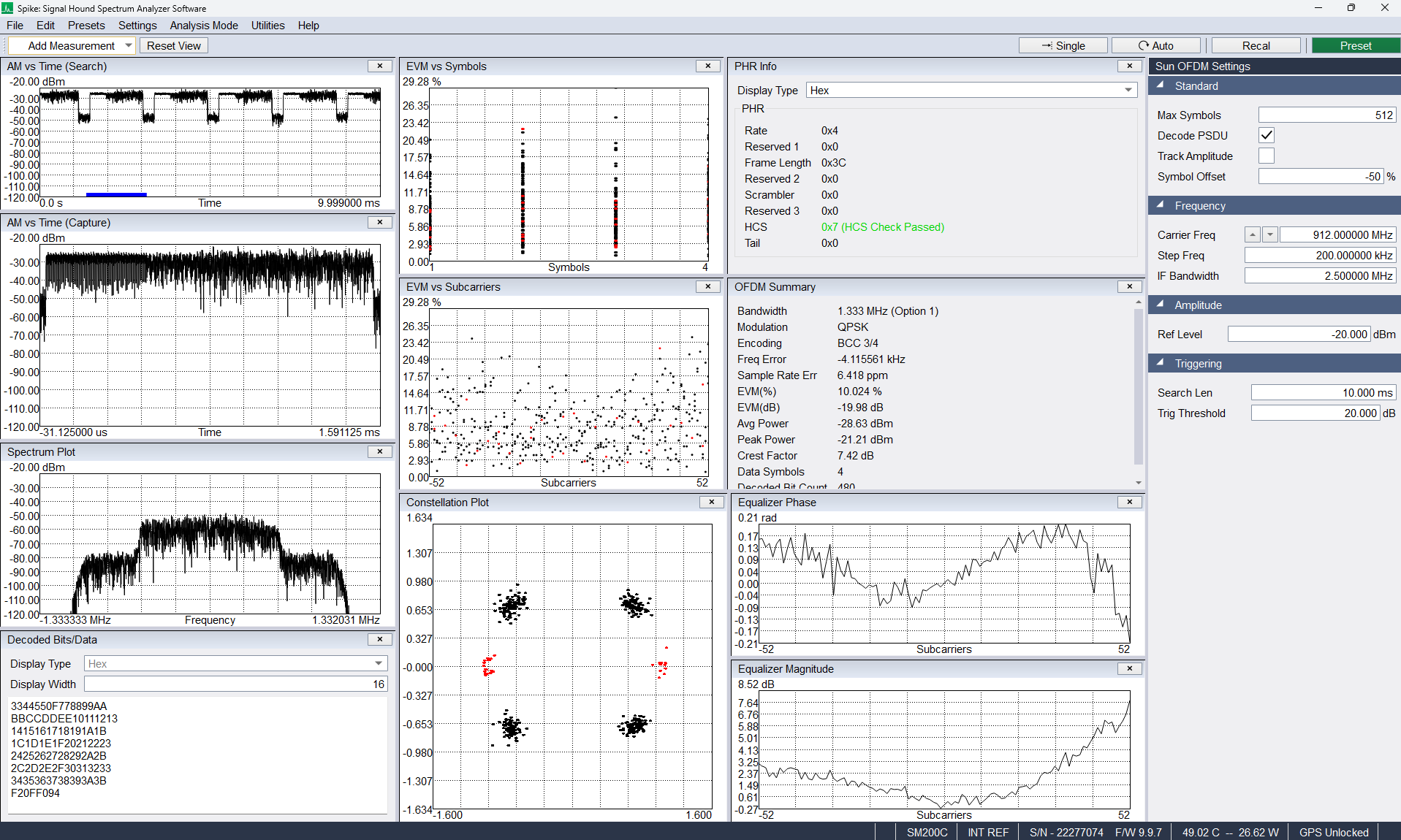
Option 1, MCS 4 SUN-OFDM Signal Demodulation
This analysis mode performs automatic detection and demodulation of waveforms adhering to the 802.15.4-2024 SUN OFDM PHY specification.
The software supports the following PHY capabilities
- All options/bandwidths [1-4]
- The signal option/bandwidth is automatically detected.
- All MCS values [0-6]
- phyOfdmInterleaving = 0 only
Supported Devices
The SUN-OFDM PHY specifies a maximum bandwidth of 1.2 MHz. To perform these measurements, the spectrum analyzer must have at least 1.2 MHz of instantaneous bandwidth.
| Device | Maximum Expected SNR |
| SM200/435 | 50 dB |
| SP145 | 50 dB |
| BB60 | 35 dB |
Measurement Concepts
The detection and demodulation procedure is described below,
- The software captures data equal in length to the user-specified Search Len (the search window).
- A sliding average power window is ran over the windows to find the leading edge of a packet. The OFDM threshold controls the sensitivity of this power detector.
- Symbol timing is determined from the STF.
- Frequency offset is determined from the STF and LTF.
- The option is detected using the STF/LTF.
- The equalizer is calculated from the LTF.
- The PHR is demodulated and decoded.
- The PSDU is demodulated and decoded (if enabled).
- Pilot tracking over the PSDU corrects residual frequency, sample rate, and amplitude error.
Triggering
A measurement is not triggered until a valid packet demodulation occurs.
Measurement Control Panel
- Max Symbols - Maximum number of symbols to demodulate. If the number of detected symbols exceeds this value, demodulation will stop at this number of symbols and the decoding of bits will not occur.
- Decode PSDU - When enabled, the PSDU is decoded and the payload data is shown in the decoded bit view.
- Track Amplitude - When enabled, the pilot tones are used to correct the amplitude for each symbol, correcting amplitude droop or fluctuations throughout the transmission.
- Symbol Offset - Symbol offset as a percentage of the guard interval. Valid range is -100 to 0. Example, -75 samples the symbol halfway 25% into the guard interval.
- Carrier Freq - Center frequency of the measurement.
- Step Freq - Frequency step size for the up/down frequency buttons.
- IF Bandwidth - Baseband filter bandwidth applied before the measurement. Should be wide enough to accommodate the signal but narrow enough to reject adjacent channels.
- Ref Level - Maximum signal input level before IF overload. For OFDM, this may be several dB above the expected average power due to high PAPR. Too high a reference level reduces SNR and packet detection sensitivity.
- Search Len - Length of the waveform search window. Must be greater than the expected packet length.
- Trig Threshold - Sliding window trigger threshold for OFDM measurements. Lower values trigger on lower SNR signals at the risk of false triggers. Roughly represents the dB level above noise floor needed for packet detection.
Measurement Windows
Multiple measurement windows can be added to the application. Layouts are saved in presets and when closing the application. A description of all measurement plots is below.
AM vs Time (Search)
Shows the full waveform search period. This view is the primary view to use when troubleshooting or unable to detect a waveform.
This plot continues to update even when no signal is found, or when a invalid packet is detected. In those cases an error string is shown for troubleshooting. See Troubleshooting for more information.
On successful demodulation, the detected packet is highlighted.
AM vs Time (Capture)
On valid measurement, shows the demodulated packet envelope. Also includes some pre/post-trigger.
Spectrum Plot
Shows the spectrum of the demodulated packet. Overlapping FFTs are performed over the packet duration. A max hold detector is ran on the FFT results.
Constellation Plot
The decoded PSDU data and pilot subcarriers are displayed on the complex plane. The data shown is post equalization and pilot tracking.
OFDM Summary
Displays several common RF measurements and PHY characteristics.
EVM vs Symbols
Plots the EVM of the data and pilot subcarriers of the PSDU by symbol.
EVM vs Subcarriers
Plots the EVM of the data and pilot subcarriers of the PSDU by subcarrier.
Equalizer Magnitude
Shows the equalizer/channel magnitude response. The equalizer shown includes any corrected pilot tracking errors.
Equalizer Phase
Shows the equalizer/channel phase response. The equalizer shown includes any corrected pilot tracking errors.
PHR Info
Displays all fields of the PHR as decoded.
Decoded Bits/Data
When Decode PSDU is enabled, the decoded PSDU bits are shown here.
The tail and pad bits are not included, only the number of bytes specified in the PHR.
The bit stream is interpreted as LSB on 1 byte boundaries.
Troubleshooting
The AM vs Time (search) plot displays a number of measurement warnings and errors which provide insight on why a measurement has failed. A list of common warnings is below,
- Trigger Not Found - Power detector was not able to find any signal. Try decreasing the trigger threshold, verify the receiver is tuned to the correct frequency, or verify the transmitter is operating correctly.
- Invalid Option Detected - Unable to detect the option/bandwidth of the signal. This may occur if the frequency offset is too large, or if a different waveform was detected. The bandwidth of the measured signals should be between 200 kHz and 1.2MHz.
- Invalid Rate Detected - The rate detected in the PHR is not a valid rate.
- Invalid Number of Symbols - Shown when the PHR frame length and the packet duration (time between the rising and falling edge of the packet) are not compatible. This may be due to low SNR environments, or invalid PHR decoding.
If the HCS check fails, as indicated in the PHR info plot, this is usually a symptom of low SNR, or an invalidly formatted payload/PHR.
Bluetooth® Low Energy
The Bluetooth Low Energy (BLE) measurement mode allows general-purpose BLE measurements and testing of BLE waveforms against Bluetooth SIG transmitter test specifications. Spike performs automatic detection and demodulation of BLE waveforms, displays results in standard measurement windows, and can save decoded packets to a .pcap file for further analysis. Spike supports waveforms meeting the core 5.2 specification, 1 MHz PHY only.
Measurement Concepts
Demodulation
When Demod measurement type is selected, Spike captures I/Q data over a specified search length at the selected center frequency and searches for a valid BLE waveform. If found, full demodulation occurs, applicable transmitter tests are run, and all measurement windows (except in-band emissions) are updated.
Detection uses a moving-average power detector combined with a preamble detector. When a valid preamble is detected, the access address and PDU header are decoded. The PDU is de-whitened using the center frequency (or a manually specified channel index). The waveform is rejected if the signal length does not match the expected size from the PDU header.
Transmitter Testing
Spike performs the following transmitter tests as defined by the Bluetooth® SIG (RF-PHY.TS.p15):
- TP/TRM-LE/BA-BV-01-C – Output power
- TP/TRM-LE/BA-BV-03-C – In-band emissions
- TP/TRM-LE/BA-BV-05-C – Modulation characteristics
- TP/TRM-LE/BA-BV-06-C – Carrier frequency offset and drift
Test limits default to specification values but can be modified by the user. Modified limits persist only in user presets and do not carry over between program instances unless saved.
- Output power measurements are performed on all valid BLE waveforms.
- Carrier offset and drift measurements require PDU bits equal to the pattern 10101010 or 01010101.
- Modulation characteristic measurements require PDU bits equal to 00001111 or 11110000. Note: some measurements (e.g., f2/f1) require both 01010101 and 00001111 patterns before a valid result is produced.
- The PDU type does not need to be a test packet; any PDU type is searched.
In-Band Emissions
Activated by selecting the in-band emissions measurement type. Only the in-band emissions plot updates in this mode. A sweep is performed over the full 2.4 GHz band using the configuration from TRM-LE/BA/VB/03. The transmit channel is detected automatically by finding the highest channel power among the 40 BLE transmit frequencies.
Sweep configuration: Span = 81 MHz, RBW = VBW = 100 kHz, Detector = Average, Sweep time = 100 ms.
Control Panel
- Measurement – Select between demodulation measurements and in-band emissions.
- Channel – Quick frequency selector for demodulation measurements.
- Carrier Freq – Manual frequency selection for demodulation. When Override Ch. Index is off, the carrier frequency determines the transmit channel and PDU de-whitening seed.
- Step Freq – Amount the carrier frequency changes when using the arrow buttons.
- Bandwidth – Acquisition bandwidth for demodulation measurements.
- Override Ch Index – When enabled, the channel index can be specified manually, allowing measurements on signals generated at any frequency.
- Channel Index – Channel index used to seed PDU de-whitening when override is enabled.
- Ref Level – Maximum input power to the spectrum analyzer.
- Search Len – Length of the waveform search window. Longer values increase capture probability at the cost of measurement speed.
- Edit Test Limits – Modify transmitter test limits. Changes persist only in user presets.
- Select Save Dir – Select the default directory for PCAP files.
- Start Recording – Start PCAP recording.
Bluetooth® Low Energy Measurement Windows
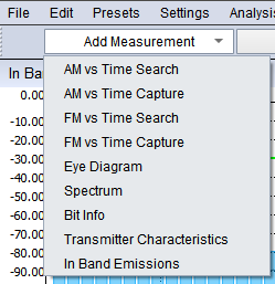
Bluetooth LE measurement plots.
Measurement windows are added to the plot area using the Add Measurement combo box.
AM vs Time Search
Shows the full waveform search period for demodulation measurements. A detected waveform is underlined in blue. This plot updates even when no signal is found, making it useful for troubleshooting and verifying signal activity. Annunciators that may appear:
- No Signal Found – The power detector did not detect a packet. Possible causes: SNR too low, or the packet started before the search window began.
- No Preamble Found – The packet leading edge did not contain a valid preamble (at least 8 alternating bits). Possible causes: SNR too low or frequency offset too large.
- Format Error Detected – The demodulated header does not match a valid pattern, or the expected payload extends beyond the packet signal. Common causes: an interfering packet mid-transmission or SNR too low.
AM vs Time Capture
Shows amplitude vs. time over the captured waveform, from the first symbol of the preamble to the last symbol of the CRC.
FM vs Time Capture
Shows frequency vs. time over the captured waveform, from the first symbol of the preamble to the last symbol of the CRC.
Eye Diagram
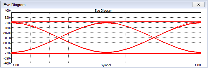
2FSK eye diagram.
Shows every FSK symbol transition in the captured waveform. Provides a quick view of signal health including frequency offset, drift, noise, filter performance, and symbol timing errors.
Spectrum
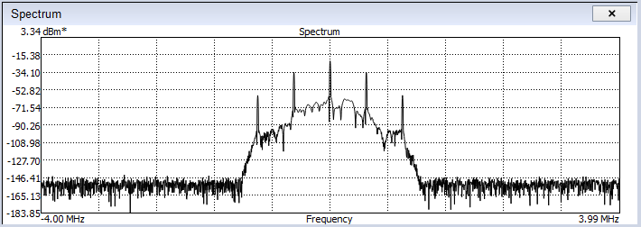
BLE spectrum
The frequency spectrum calculated over the capture interval using a Nuttall window.
Bit Info
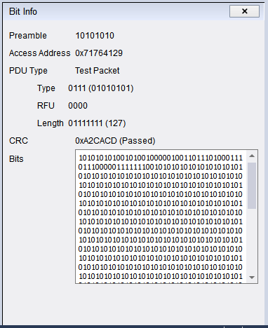
Decoded BLE packet bit info.
Displays the data components of the captured waveform. Each component of the PDU header is shown along with the bits for the entire capture. The PDU type is determined from both the current channel index and the access address value. CRC pass/fail is only shown for advertising and test PDU types.
Transmitter Characteristics
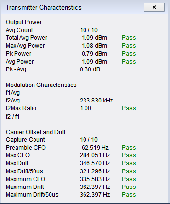
Transmitter characteristics results.
Displays all transmitter test results except in-band emissions. Results appear once a valid packet has been detected for each test and are averaged/max-held for up to 10 captures. Results reset when any configuration parameter changes or the Recal button is pressed.
In-Band Emissions
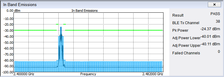
In band emission testing.
Displays the in-band emissions transmitter test results. Updated only when the measurement type is set to In-Band Emissions.
PCAP Recording
Spike can store every successfully demodulated packet into a .pcap file using the libpcap format with the LINKTYPE_BLUETOOTH_LE_LL_PHDR link-layer header type. All packets captured while Demod measurement type is active are stored when recording is running. Use the Start/Stop button on the control panel to control recording. Third-party applications are required to view the contents of .pcap files.
WLAN Modulation Analysis
The Spike software supports 802.11b/a/n/ac/ax/ah modulation analysis, performing physical layer (PHY) measurements including RF quality metrics, channel characterization, and bit-level troubleshooting. WLAN measurements are available for SM, SP, and BB series devices.
Control Panel
- Standard – Select the WLAN standard to measure. The 40 MHz standard must be selected when measuring 40 MHz signals. Bandwidth is auto-detected for AH signals.
- Max DSSS Symbols – Maximum DSSS symbols to measure (802.11b only). Packets are truncated to this length.
- Decode PSDU – When enabled, OFDM PSDUs are decoded and shown in the decoded bits view. Only BCC-encoded payloads can be decoded. Does not apply to DSSS waveforms.
- Eq Training – Specify how the equalizer is trained: Preamble uses only the long training sequence; Preamble + Data also uses the payload to estimate the channel response.
- Track Amplitude – Enable amplitude pilot tracking to adjust the channel estimate for each data symbol, correcting amplitude fluctuations throughout the transmission.
- Symbol Offset – (OFDM only) Symbol offset as a percentage of the guard interval (range: −100 to 0, default: −50%). −50% samples the symbol halfway through the guard interval. Auto-adjusted for short GI.
- 2.4 GHz Ch. / 5 GHz Ch. – Select a carrier frequency by industry-defined channel number.
- Carrier Freq – Center frequency of the measurement. For OFDM, this should be the center-most null DC subcarrier frequency. Must be within ±624 kHz for 20/40 MHz OFDM or ±2.7 MHz for DSSS.
- Step Freq – Frequency step size for the up/down frequency buttons.
- IF BW – Baseband filter bandwidth applied before the measurement. Should be wide enough to accommodate the signal but narrow enough to reject adjacent channels.
- Ref Level – Maximum signal input level before IF overload. For OFDM, this may be several dB above the expected average power due to high PAPR. Too high a reference level reduces SNR and packet detection sensitivity.
- Meas Filter – DSSS pulse shaping filter (currently fixed as rectangular window).
- Filter Bbt – Pulse shaping filter coefficient (not currently used with rectangular window).
- Search Len – Length of the waveform search window.
- OFDM Trig Threshold – Sliding window trigger threshold for OFDM measurements. Lower values trigger on lower SNR signals at the risk of false triggers. Roughly represents the dB level above noise floor needed for packet detection.
- DSSS Trig Level – Absolute video trigger level for DSSS measurements. Use the AM vs Time (Search) window to estimate a valid level.
Measurement Windows
Multiple measurement windows can be added to the application. Most target either OFDM or DSSS modulations. A quick-setup button switches between OFDM and DSSS window configurations, and layouts can be saved through presets.
AM vs Time (Search)
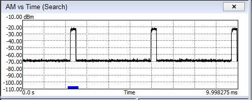
AM vs time window with highlighted 802.11 measurement interval.
Shows the full waveform search period. Detected waveforms are underlined in blue. Updates even when no signal is found, making it useful for troubleshooting.
Decoded Bits/Data
When the PSDU is BCC encoded and Decode PSDU is selected, decoded bits are shown here. For non-802.11ax waveforms, leading service bits and trailing zero bits are discarded. For 802.11ax, all bits up to the post-FEC bits are displayed.
MAC Header Info
Shows the decoded payload as a MAC header. Valid only for non-aggregate payloads.
Symbol Table
Shows transmitted bits for an OFDM waveform. Each OFDM symbol appears on a separate row. Only data and pilot subcarriers are shown; pilot subcarriers are highlighted in red.
Measurement Concepts
Search Window
Spike acquires data equal in length to the user-specified search length (the search window) and searches for a valid packet within it. The packet must be fully contained in the search window. The search length should be sufficiently larger than the expected packet length. Only one measurement is performed per search window.
802.11 a/n/ac/ax Demodulation
- A sliding average power window (OFDM threshold) finds the leading edge of the transmission.
- Symbol timing is performed using the L-STF.
- Frequency offset is measured and corrected using the L-STF and L-LTF.
- Equalization for the L-SIG uses both L-LTF symbols with an averaged zero-forcing algorithm. PSDU equalization uses a zero-forcing algorithm on the LTF sequence before data symbols.
- Symbols are demodulated using the configured symbol offset (default −50%).
- Pilot tracking over the PSDU corrects residual frequency offset and sample rate offset.
- The PSDU is decoded if Decode PSDU is enabled and BCC encoding is used. LDPC-encoded PSDUs are not decoded.
802.11 AH Demodulation
Bandwidth is auto-detected. Demodulation follows similar steps: power-based packet detection, STF timing, bandwidth detection (1/2/4/8 MHz), LTF fine timing, frequency correction, LTF-based zero-forcing equalization, symbol demodulation at the configured symbol offset, pilot tracking, and optional BCC PSDU decoding.
DSSS Demodulation
Signal detection uses a user-supplied video trigger with hysteresis, followed by a preamble detect for synchronization. Full demodulation uses standard BPSK/QPSK techniques.
WLAN Measurement Walkthrough
- Use sweep mode to find a WLAN signal of interest and center on it.
- Switch to WLAN mode via Analysis Mode. The center frequency and reference level carry over.
- The default layout is preset for OFDM with the 802.11a standard selected. If no measurement appears, check the AM vs Time (Search) window for an error status.
- If Trigger Not Found is shown, compare the trigger level setting against the signal amplitude visible in the search window and lower the trigger level accordingly.
- Select the correct standard (e.g., 802.11n 20 MHz), adjust the carrier frequency if needed, and set the reference level above the maximum expected signal power.
- Set the trigger level and search length. Use the AM vs Time (Search) plot to estimate a valid trigger level.
- Once settings are correct, other windows begin updating and the AM vs Time (Search) plot shows a blue bar under the detected signal.
- Press Single to force one additional valid measurement.
- Add measurement windows with the Add Measurement menu and save the configuration via presets.
Troubleshooting
- Invalid Packet Format – The triggered measurement could not be demodulated using the current standard. Check that the correct standard is selected and that the signal is not too impaired.
- Not Enough Samples – The waveform was detected near the end of the search window. Increase the search length.
- Trigger Not Found – Verify the signal is present in the search window and that the trigger level is appropriate for the observed signal levels.
- Use the IF Bandwidth control to reject out-of-channel signals from adjacent WLAN or Bluetooth® sources.
- The BB60C/D can only measure 20 MHz BW OFDM waveforms.
LTE
LTE measurements require the correct MATLAB® runtime libraries. See the Appendix for installation instructions. LTE measurements are supported on 64-bit Windows and Linux only.
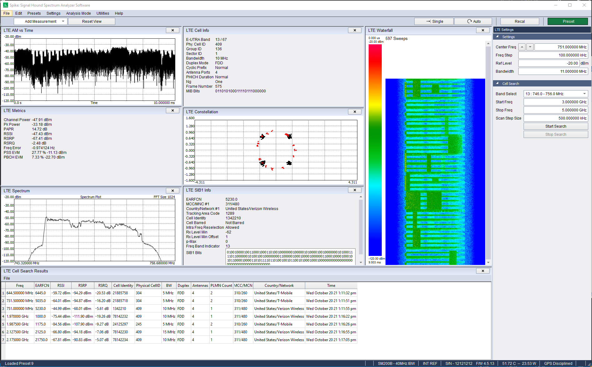
LTE measurements are available for SM, SP, and BB series devices. Spike provides basic downlink cell measurements including cell search, scanning, and the following:
- Cell search and measurement at a specified center frequency.
- Cell scanning over a range of frequencies and LTE bands (detected cells aggregated in a results window).
- Automatic MIB decoding: Physical Cell ID, bandwidth, duplex mode, frame configuration.
- Power measurements: RSSI/RSRP/RSRQ, frequency error, EVM for PBCH and PSS, PAPR.
- Automatic SIB1 decoding: MCC/MNC pairs with country/provider lookup, EARFCN, TAC/Cell Identity.
- Standard spectrum plots: AM vs Time, Spectrum, Waterfall, Constellation for PBCH and PSS.
Measurement Concepts
Spike supports two LTE acquisition modes:
- Single frequency – Analyzer is tuned to a specific frequency; cell search and full synchronization/demodulation occur at that frequency. Best for transmitter testing or characterizing a single cell.
- Cell scanning – Software scans user-configured frequencies/bands. At each frequency, cell search occurs; if a cell is found, full synchronization and demodulation are performed and the result is added to the cell search results table before advancing to the next frequency.
Cell Detection
Spike uses the PSS and SSS for cell search. The cell must be within ±7.5 kHz of the selected center frequency. A successful PSS/SSS detection determines duplex mode, cyclic prefix length, and triggers MIB decoding.
If any step from cell search to MIB decoding fails, the measurement fails and an error code is reported. If the MIB is decoded successfully, Spike attempts SIB1 decoding. The SIB1 is transmitted on even-numbered frames; if the detected frame is odd, Spike looks at the next frame. SIB1 decoding failure results in a valid measurement with SIB1 fields left empty.
The full process uses approximately 40 ms of captured I/Q data at the highest available bandwidth to support all possible cell bandwidths. In single-frequency mode, the reference level is user-specified. In scan mode, Spike starts in the most sensitive configuration and increases the reference level if IF overload occurs.
Control Panel
- Center Freq – Measurement center frequency for single-frequency mode. Not used during cell scans.
- Freq Step – Frequency step when using the center frequency arrow buttons.
- Ref Level – Measurement reference level for single-frequency mode.
- Correlation Threshold – Cell search correlation threshold (0.0 to 1.0).
- Include in Results – When enabled, single-frequency measurements are added to the cell search results list.
- Configure Scan – Opens a dialog for selecting bands for the cell scan. The Scan Info label summarizes the configured bands.
- Scan Type – Single: one pass through all configured bands. Continuous: repeats until Stop Scan is pressed or the mode is exited.
- Sort By – Sort order for the cell search results table: RSSI, frequency, or time.
- Keep – When result grouping is enabled and a duplicate cell is detected, determines whether to show the most recent measurement or the highest-power measurement.
- Group Results – When enabled, results with matching frequency and Physical Cell ID are grouped as a single cell.
- Split PLMNs - When enabled, each PLMN detected in a measurement is given its own row. The PLMN count is set to 1 for each row generated. When enabled, grouping will then occur on frequency, Cell ID, and MCC/MNC.
- Max Results – Maximum number of cells shown in the cell search results table.
- Start Scan / Stop Scan – Start or stop a band scan.
Cell Search Results
The cell search results window collects scan results and, if enabled, single-frequency measurement results in an ordered list. Results can be grouped, sorted by frequency/amplitude/time, cleared, accumulated across multiple scans, exported to CSV, or exported to a custom format that can be re-imported into Spike.
Mapping
Mapping mode binds measurements to geolocations. Features include
- Compound measurements
- Georeferenced map import
- GPS integration
- Manual and Automated measurements
- Heat mapping
- Grid testing
- Report generation
- Direction finding via visual triangulation
- Audio RSSI
- Session import/export
- KML export for Google Earth compatibility.
Measurements
Compound Measurements
Multiple frequencies or channels can be monitored simultaneously using the compound measurement functionality. Compound measurements allow multiple fully independent measurements to be configured. Each configuration can be separately stored and viewed on the map. All configured measurements are performed sequentially each time a measurement is configured. The Measurements Editor (opened via Configure Measurements in the Meas Settings control panel) defines the list of configured measurements.
Channel Power
The channel power measurement is the main measurement performed in mapping mode. Channel power measures the power of a modulated/broadband signal over the user defined frequency span.
The channel power results include power, peak power, and occupied bandwidth.
LTE
Performs a single-frequency cell search and measurement. This measurement only supports downlink LTE signals up to 20MHz bandwidth.
The LTE result is selectable as RSSI or RSRP. See LTE for details.
(Requires MATLAB® runtime; 64-bit Windows and Linux only.) See MATLAB® Runtime Installation Instructions.
Measurement Settings Control Panel
- Active Meas – Selects which measurement configuration and corresponding points are shown in the map, spectrum, and table views.
- Configure Measurements – Opens the Measurements Editor for managing compound measurements.
Point Settings
- Declination – Adjustment for magnetic declination in degrees, applied to angles entered in the Azimuth field for a point's detail view.
- Occupied Bandwidth – Percentage power used in the occupied bandwidth calculation.
- GPS Meas Speed – Minimum time elapsed since the last measurement before a new one is taken.
- GPS Meas Min Delta – Minimum distance from the location of the last measurement before a new one is taken.
- Max Points – Maximum number of measurements that can be acquired. Does not retroactively affect existing measurements.
- Clear Points – Clears all measurements (confirmation dialog shown).
Audio Settings
- Audio Enabled – Enables RSSI audio tone using the system audio configuration. Tone frequency increases with measured channel power.
- Volume – Volume of the audio tone.
Plot Settings
- Map – Shows or hides the map view.
- Spectrum – Shows or hides the spectrum plot of the current measurement.
- Measurements Table – Shows or hides the measurements table.
Grid Settings
- Grid Enabled – Enables or disables grid testing. When enabled, the grid appears in the map view, grid test results appear in the Grid Table, and the report includes those results.
- Rows / Columns – Number of rows and columns in the grid.
- Horiz Offset / Horiz Scale – Horizontal position and width of the grid.
- Vert Offset / Vert Scale – Vertical position and height of the grid.
Report Settings
- Configure Report – Opens a dialog for editing report metadata (report number, date, test engineer, notes).
- Generate Report – Opens a save dialog to export a PDF report of the current session.
Session Settings
- Autosave Sessions – When enabled, a new timestamped session is automatically saved each time the unsaved point count reaches the autosave interval.
- Autosave Interval (Points) – Number of measurement points that can accumulate before autosave triggers.
- Change Directory – Specify the directory where sessions are automatically saved.
- File Prefix – Prefix for autosaved session files.
Measurements Editor
Manages measurement configurations/compound measurements. All configurations are performed serially when a measurement is triggered. Changing any configuration other than grid settings clears existing session points (confirmation dialog shown).
- Name – Name of the measurement configuration.
- Include in Report – Controls whether this configuration's measurements appear in the report.
- Add Meas – Adds a new configuration with default settings.
- Duplicate Meas – Adds a copy of the selected configuration.
- Delete Meas – Removes the selected configuration.
- Save Table / Load Table – Save or load the configuration list as a CSV file.
- Clear Table – Clears all measurement configurations.
- OK – Applies the configuration list (confirmation required if changes affect existing points).
- Cancel – Exits without applying changes.
Receiver Settings (common to all measurement types)
- Center Freq – Center frequency of the measurement.
- Ref Level – Controls the sensitivity of the receiver. Should not be lower than the maximum expected input level. Also sets the top line of the graticule of the spectrum plot.
Measurement Settings
- Type – Measurement type.
- Channel Power — Meas Bandwidth: bandwidth of the channel power measurement.
- LTE — LTE Meas Type: type of LTE measurement (RSSI or RSRP).
Sweep Settings
- Span – Frequency span around the center frequency.
- RBW / VBW – Resolution and video bandwidth (flat-top window).
- Auto RBW / Auto VBW – Automatically select RBW and set VBW = RBW.
Grid Settings
These settings are used to define acceptance criteria for grid testing via upper and lower amplitude thresholds
- Use Lower Threshold / Lower Threshold – Enable and set a minimum amplitude value for a grid cell to pass.
- Use Upper Threshold / Upper Threshold – Enable and set a maximum amplitude value for a grid cell to pass.
Map Settings Control Panel
- Map Scale – Zoom percentage of the map.
- Heatmapping – Selects basic or advanced heatmap display.
- Points Visible – Shows or hides measurement points and heatmap.
- Point Border – Toggles a black border around points.
- Point Size / Point Opacity – Size and color opacity of points on the map.
- Azimuth Lines – Toggles lines drawn from directional points at their azimuth angles (basic heatmap only).
- Min Color / Max Color (dBm) – Power values mapped to the coldest and hottest colors. Max Color cannot exceed the reference level.
- Auto Color – Automatically maps the heat color range to the min/max power across current points.
- Grayscale – Renders the heatmap in grayscale.
Map View
An interactive georeferenced map with overlaid measurements and controls. Load a map image via File > Load Map, then georeference it via File > Set Coordinates by entering the bounding latitude (top/bottom) and longitude (left/right) coordinates. Remove the map with File > Unload Map (clears all measurements and coordinates). See the OSM Map Import Guide for instructions on importing maps from OpenStreetMap.
If GPS data is available (internal or external), the user's current location is shown as a red target icon. See GPS Control Panel for configuring the GPS.
Three interaction modes (selected via icon buttons in the upper toolbar):
- Select mode (arrow icon) – Click to select/deselect points. Selected point details appear in the detail panel. Directional point azimuths can be changed by dragging.
- Click mode (pencil icon) – Click on the map to capture a measurement at the cursor location.
- GPS Tracking mode (GPS paddle icon) – Available when GPS is connected. Measurements are taken automatically at the intervals specified by GPS Meas Speed and GPS Meas Min Delta.
Color Bar
Shows the hot-to-cold color spectrum and the corresponding dBm values at the top and bottom. Configured via Min Color and Max Color sliders, or automatically set by Auto Color.
Measurement Detail Panel
The measurement detail panel appears whenever a point is selected, and shows all the details of that measurement. They are:
- Frequency – The center frequency at the time of measurement.
- Bandwidth – The meas bandwidth at the time of measurement.
- Power/RSSI/RSRP – The measured channel power, RSSI, or RSRP of the signal.
- Peak – The measured peak power of the signal.
- Occupied/Cell Bandwidth – The measured occupied or cell bandwidth of the signal.
- Time – Timestamp for when the measurement occurred.
- Latitude – The latitude dimension of the point’s geocoordinates.
- Longitude – The longitude dimension of the point’s map coordinates.
- Pixels from Left – The horizontal position of the point on the currently loaded map.
- Pixels from Top – The horizontal position of the point on the currently loaded map.
- Directional – Whether or not the point has a directional component.
- Azimuth – The direction or bearing of the point, specified as an angle in degrees clockwise from North, from 0 to 360. If a declination is set in the Declination field of the Meas Settings control panel, then it will be automatically
Sessions
A session includes a georeferenced map image, a set of measurement points, and a preset storing measurement and map configurations. Sessions are saved as three files: a .spikemap (JSON measurements and map config), a .png (map image), and an .ini (measurement configuration preset). All three files must stay in the same directory when moved.
Import/export sessions via File > Import Session and File > Export Session.
Spectrum Plot
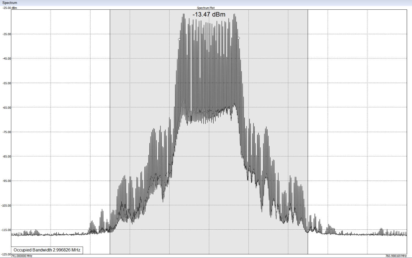
Channel power measurement within the mapping spectrum plot.
- Channel Power – Shows the current sweep with the channel power measurement window shaded and diamonds marking the occupied bandwidth bounds. Channel power reading is displayed top-center; occupied bandwidth is shown bottom-left.
- LTE – Shows the LTE measurement with the cell bandwidth shaded when a valid cell is detected.
Measurements Table
Points Table
Displays all measurements captured in the current session. Export options:
- CSV – Points saved as a CSV file.
- KML – Points saved in KML format (XML-based geodata compatible with Google Earth and Google Maps). Measurement details are compiled in an HTML table within the description field; heat mapping is visible in Google Earth.
Grid Table
The grid table displays aggregate information for each grid cell, including the grid index number, pass/fail status, number of points contained by the cell, worst power measured in cell, margin of error (passing cells have positive margins), average power measured in cell, and measurement configuration details.
The table can be exported as a CSV file with File > Save CSV.
Opening a KML file in Google Earth
To open a KML file of measurement points saved with the File->Save KML menu item, open Google Earth in a web browser. Click the Projects icon, then click the New Project button, and then choose Import KML File from Computer.
Audio Received Signal Strength Indicator (RSSI)
An audio tone tracks channel power. When enabled, tone frequency rises with signal power. Toggle and set volume in Audio Settings in the Meas Settings menu.
Grid Testing
For indoor testing, a grid divides a floorplan into cells, aggregates measurements in each cell, and tests them against the thresholds set in each measurement configuration.
Enable grid testing and configure the grid using the controls in the Grid Settings section of the Meas Settings control panel.
Upper and lower test thresholds are set for each measurement configuration in the Grid Settings section of the Measurements Editor.
The grid is overlaid on the map. Each cell has a unique index number displayed in its upper left corner, which corresponds to the cell number in the grid table. Each cell displays the worst amplitude seen within it in the center, and is colored green for passing and red for failing. Cells with no valid measurements within them are not colored.
Report Generation
Reports can be generated in the form of PDF files. Reports contain general information such as date, device, and operator, as well as sections for each measurement configuration. For each configuration, reports show pass/fail status if grid testing is enabled, measurement settings, a measurements table, and map image.
If grid testing is enabled, then the measurements table will replicate the grid table in the user interface. Otherwise, it will replicate the points table.
VCO Characterization
VCO Characterization mode evaluates the performance characteristics of voltage-controlled oscillators (VCOs), including frequency vs. voltage, sensitivity (Hz/V), power vs. voltage, current vs. voltage, and harmonic power vs. voltage for the first six harmonics. Requires a PN400 phase noise tester. Available for SM, BB, and SP145 series devices.
VCO Settings Control Panel
PN400 Settings
- Status – Indicates whether a PN400 is connected.
- Connect – Connect a PN400 device.
DC Source Settings
- Enable Output – Master enable for PN400 DC outputs. When disabled, no DC power is emitted.
- Fixed V Supply – Level of the fixed V Supply output.
Sweep V Tune Settings
- Start / Stop – Starting and stopping control voltages for the sweep.
- Meas Points – Total number of voltage points to measure.
- Dwell Time – Delay between setting the PN400 output voltages and measuring the VCO response.
Meas Settings
- Ref Level – Power level of the top graticule line. Should not be lower than the maximum expected VCO output level.
- Auto Freq Band – Automatically determine the frequency range for measurements.
- Freq Start / Freq Stop – Start and stop frequency for each measurement.
- Freq Resolution – RBW of the analyzer sweep at each measurement point.
- Channel Power Width – Width of the channel for power and harmonics measurements.
DC Limits Settings
- V Tune Min / Max – Minimum and maximum output voltage of the V Tune port on the PN400.
- V Supply Min / Max – Minimum and maximum output voltage of the V Supply port on the PN400.
Measurement Windows
- Frequency – Frequency vs. voltage plot showing the VCO's peak output frequency at each control voltage.
- Sensitivity – Slope of VCO performance: frequency change between measurement points in Hz/V.
- Power – Power vs. voltage plot showing VCO output power at each control voltage.
- Current – Current vs. voltage plot showing VCO supply current at each control voltage.
- Harmonics – Harmonic power vs. voltage plot showing VCO output at each of the first six harmonics for each control voltage.
VCO Characterization Measurement Walkthrough
When entering VCO Characterization mode, Spike automatically searches for a connected PN400. If found, the Status field in the PN400 section shows the serial number in green. If not, a dialog prompts the user to connect a PN400 and press Connect.
The mode remains idle until Single is pressed to begin a measurement. Configure all settings before pressing Single.
DC power on the PN400 is disabled by default. To avoid VCO damage, set appropriate V Tune and V Supply limits in the DC Limits section before enabling output in the DC Source section.
At each voltage point (from Start to Stop), the PN400 V Tune port is set to the target voltage, execution is delayed by the dwell time, and the analyzer sweeps the configured frequency band. The peak sweep value determines the frequency measurement. Sensitivity is derived from the frequency change between the current and previous point. Power and harmonic measurements use channel power measurements around the peak and the first six harmonics at the configured channel power width. Current is reported directly by the PN400.
A measurement can be aborted at any time with the Abort button. Changing configuration during a measurement restarts the measurement with the new settings.
Pulse Analysis
Pulse analysis provides tools for detecting and characterizing pulsed RF signals, compatible with all Signal Hound receivers (analysis bandwidths up to 160 MHz). Features include:
- Automatic detection and characterization of CW, Chirp, and Barker pulse types.
- Deep pulse history of >50,000 pulses.
- Detailed pulse metrics per IEEE 181-2025.
- Configurable plots: AM/FM/PM vs Time, Spectrum/Waterfall, Histograms, Pulse Tables, Pulse History, Pulse Compression, Auto-Correlation.
- Deinterleaving — classify signals from unique emitters.
- Pulse correlation/compression testing against a reference waveform.
Acquisition
Pulse analysis captures contiguous I/Q snapshots triggered by video, external, or free-running trigger.
Capture Settings
- Ref Level – Controls instrument sensitivity. Maximum pulse amplitude should not exceed this value.
- Center – Center frequency of the I/Q snapshot.
- Step – Frequency step for the Center up/down arrows.
- Sample Rate – I/Q sample rate of the snapshot.
- IF Bandwidth – I/Q bandwidth of the snapshot.
- Auto IFBW – Automatically select bandwidth based on sample rate.
- Search Windows – Length of the I/Q snapshot.
Trigger Settings
- Trigger Type – Select the trigger type (video, external, or free-running).
- Trigger Edge – Rising or falling edge (video and external triggers).
- Trigger Position – Percentage into the snapshot at which the trigger occurs.
Pulse Detection
Once an I/Q snapshot is collected, pulses are detected using the trigger level to identify rising edges. A list of viable pulses is assembled and characterized. Pulses not meeting user-configured requirements are discarded.
Accumulated Pulse Results
When enabled, all valid pulses are added to the accumulated results — a running list from the last several snapshots. When full, the oldest pulse is removed as each new one is added. Pulse history plots display accumulated pulse results.
Detection Settings
- Trigger Level – Used for pulse detection and, if enabled, video triggering.
- Max Pulse Count – Maximum pulses detected per I/Q snapshot. Additional detected pulses are discarded.
- Selected Pulse – Which pulse to display on Pulse View plots.
- Accumulate Results – When enabled, stores all detected pulses in the accumulated results.
- Max Accumulated – Maximum size of the accumulated results.
- Clear on Reconfigure – When enabled, clears accumulated results whenever the measurement configuration changes.
- Pulse Meas Count – Number of pulses detected in the current I/Q snapshot.
- Pulse Accum Count – Number of pulses in the accumulated results.
- Clear Accumulated – Clears all accumulated pulse results.
Plots
Measurement Views
Operate on the I/Q snapshot. Time-domain views highlight and number detected pulses. The spectrum plot uses overlapping max-held FFTs across the full snapshot; FFT size and count are set in the spectrum settings. All spectrum FFTs are also shown in the waterfall display.
Pulse Views
Operate on a single pulse selected by Selected Pulse in the detection settings. The pulse is padded by 10% of its width.
Pulse Tables
Tabulate characteristics of all detected pulses — one table for the current snapshot and one for accumulated results. Export the full table to CSV via the file menu within the pulse table.
Histograms
View histograms of pulse width, frequency offset, amplitude, rise time, fall time, and PRI. Each characteristic's full range is divided into 100 bins and pulses are accumulated. Standard histograms operate on one snapshot; Accumulated Histograms operate on the accumulated results.
Pulse History
Plots key pulse characteristics over time using accumulated results (or current measurement if accumulation is disabled). All pulses carry high-resolution timestamps for accurate relative measurements across the full accumulated result table.
Correlation Results
Display normalized cross and auto-correlation results. Y-axis ranges from 0 (no correlation) to 1 (perfect correlation); x-axis mirrors the I/Q snapshot.
Deinterleaving
Deinterleaving identifies pulse emitters and classifies each pulse to a specific emitter. Emitters can be configured, each defined by center frequency and pulse width. Each pulse is compared to all configured emitters and a similarity score [0, 1] is calculated. If the score exceeds the deinterleaving threshold, the pulse is attributed to that emitter; if no score crosses the threshold, the pulse is unclassified.
Auto emitter detection uses a clustering algorithm on the accumulated results for both frequency and pulse width. Emitter assignments and similarity scores appear in the pulse tables; several plots color-code pulses by emitter.
Correlation
Cross Correlation
When enabled, I/Q snapshots are cross-correlated with a reference pulse (copied from a measured pulse or imported from a CSV file). The normalized output shows similarity between the reference and the snapshot, providing: pulse compression performance evaluation, at-a-glance pulse similarity detection, and detection of known low-level pulses that cannot be detected via normal triggering.
The I/Q snapshot and reference pulse should use the same sample rate. No resampling is performed — imported references must be pre-resampled.
Auto Correlation
When enabled, the beginning of the I/Q snapshot (length set by the autocorrelation time in the measurement config dialog) is autocorrelated against the entire snapshot. This reveals: periodic structures in the snapshot (PRI measurable with markers), signal regularity, and low-level unknown repeating structures not detectable through normal pulse detection.
The autocorrelation time must be longer than any periodic structure to be measured.
Measurement Configuration Dialog
Detection Tab
- Detect Chirp – When enabled, pulses with frequency deviation exceeding the chirp threshold are classified as chirp.
- Detect Barker – When enabled, each pulse is correlated with all positive Barker sequences. If the result exceeds 0.5 normalized cross-correlation, the pulse is assigned the Barker type.
- Pre-Trigger Holdoff – Time the signal must remain below the trigger level before detection.
- Ignore Dropouts – Time a pulse can droop below the trigger level without being considered ended.
- Enable Min Pulse Width / Min Pulse Width – When enabled, pulses shorter than this value are discarded.
- Max Pulse Width – Pulses exceeding this value are always discarded.
Analysis Tab
- Rise Lower / High Threshold – Start and end of the rising edge transition.
- Fall Lower / High Threshold – End and start of the falling edge transition.
- Pulse Width Threshold – Point on the transition at which pulse width is determined.
- Region Ripple – Percentage of the pulse (from center) used for ripple calculation.
- Region Linear FM – Percentage of the pulse (from center) used for frequency slope calculation.
- Chirp Threshold – Peak-to-peak frequency threshold for chirp classification (requires Detect Chirp enabled).
Deinterleaving Tab
- Deinterleaving – Enables or disables deinterleaving.
- Detection Threshold – Threshold for associating a pulse with an emitter.
- Emitter Enabled / Frequency / Pulse Width – Enable and define each emitter's center frequency and pulse width.
- Pulse Color – Color used to display pulses for each emitter classification.
- Auto Detect Emitters – Runs a clustering algorithm on accumulated results to detect emitters automatically.
- Max Emitters to Detect – Maximum number of emitters the auto-detect algorithm can find.
Correlation Tab
- Cross Correlation Enabled – Enables cross correlation (requires a loaded reference pulse).
- Import Reference Pulse – Load a reference pulse from a CSV file (ASCII floating-point I/Q pairs, one per line, I and Q separated by a comma).
- Export Reference Pulse – Export the current reference pulse to CSV.
- Save Pulse to Reference – Save a currently measured pulse (specified by Pulse #) as the cross-correlation reference.
- Clear Reference – Clear the reference pulse.
- Status / Samples – Shows whether a reference pulse is stored and its sample count.
- Auto Correlation Enabled – Enables or disables auto-correlation.
- Auto Correlation Time – Select the autocorrelation length.
Pulse Signal Definitions
Pulses are expected to conform to the single positive pulse waveform defined in IEEE 181-2025. A pulse is defined by a rising and falling transition. All threshold percentages are configurable in the Measurement Configuration Dialog.
Measurement Concepts
Measuring Frequency and Amplitude
Using Markers
Six markers are available, each with its own reference. To activate a marker, left-click inside the graticule or press Peak Search to place the marker on the current trace peak. Once active, the frequency and amplitude readout appears in the upper right corner of the graticule. Marker accuracy depends on span and RBW — narrower settings yield higher accuracy. Amplitude accuracy is independent of the dB/div setting. Reposition the marker by clicking the graticule or using the left/right arrows to shift one sample point at a time.
Using the Delta Marker
With a marker active, click Delta on the marker/trace control panel to place a reference point. The marker readout then shows the difference between the current marker position and the reference. Press Delta again to disable it.
Measuring Low Level Signals
Set the reference level to −50 dBm or lower to enable the highest sensitivity settings. Use an external timebase and a narrow span (1 kHz or less) for best results. Video averaging may be required for a stable amplitude reading.
Sweep Record and Playback
Spike can store and play back sequences of sweeps from any Signal Hound spectrum analyzer. Sweep recording files use the .shr extension.
Version 3.1.13 introduced the SHR format and can play back the older BBR format. The software no longer generates BBR files as of version 3.1.13.
Sweep Recording
The Sweep Recording control panel is available in sweep and real-time analysis modes. Two decimation methods are available to manage file size:
- Decimation in time – Averages or max-holds multiple sweeps over a configured time or sweep count before storing the result. For example, a 1-second max-hold decimation stores one max-held sweep per second.
- Decimation in frequency – Channelizes the sweep using channel power measurements. Channel width and center frequency are configurable; results can be stored in dBm or dBm/Hz. Both decimation types can be used simultaneously — channelization occurs before time decimation.
File size can also be limited using maximum file size and maximum file count settings. Press Start Recording to begin; a new sequentially numbered file is created when the max file size is reached. Press Stop Recording to end the session.
When limit lines are enabled only the sweeps that contain data that exceed the limit lines are saved.
Sweep Playback
Press the play icon on the Sweep Playback control panel and select a valid .shr file. Use the slider bar, pause, step, and rewind buttons to control playback. Playback speed sets the delay between successive sweeps (e.g., 1 second = one sweep per second). All measurement features remain active during playback (markers, min/max/avg traces, channel power, persistence, spectrogram). Press the stop icon to return control to the connected analyzer.
I/Q Recorder
The I/Q Recorder utility performs dedicated short- to long-term I/Q captures to disk. Access it via Utilities > I/Q Recorder. It provides device and file configuration, a spectrum preview window with adjustable RBW, and informational readouts during capture.
Configuration
Capture
- Center Freq – Tuned center frequency of the capture (0 Hz frequency of the I/Q data).
- Ref Level – Expected input power. Controls the reference level, gain, and attenuation.
- Sample Rate – Sample rate of the capture (device rate divided by the decimation value).
- Bandwidth – Bandwidth of the passband filter. Cannot exceed the Nyquist frequency.
- Auto Bandwidth – When enabled, passes the full I/Q capture bandwidth automatically.
Preview
- RBW – Desired RBW for the spectrum preview plot. If the FFT window length is insufficient for the desired RBW, a warning is shown.
File
- Save Directory – Directory for storing I/Q waveform files.
- File Prefix – Prefix applied to all saved file names. By default the name includes a second-resolution timestamp and sequence number.
- Max File Size – Maximum data to store in a single file.
- Max Files – Maximum number of files to write.
- Max Disk Usage – Maximum percentage of the hard disk that can be used (determined by the Save Directory). Default is 80%.
- Data File Format – File format for I/Q data. Default is binary 16-bit complex integers.
- Center Freq In Name / Sample Rate In Name – Insert the center frequency or sample rate into the file name.
Informational
- Data Saved – Total data written during the current capture.
- Files Saved – Number of files written during the current capture.
- Disk Free – Percentage of the hard disk remaining.
- Rate – Current data capture and write rate.
Recording
Press Record to begin. Data is saved to sequentially labeled files in the Save Directory, each prefixed with the File Prefix followed by a second-resolution timestamp tied to the start of the capture. Recording stops when:
- The user presses Stop.
- Max Files have been written.
- Disk usage would exceed Max Disk Usage.
I/Q File Formats
16-Bit Binary
Signed 16-bit complex integers, little-endian, stored sequentially as I1, Q1, I2, Q2 … In, Qn. Values range from −32768 to +32767 (full scale = ±1.0).
To convert to floating point:
float re32f = (float)re16s / 32768.0;
float im32f = (float)im16s / 32768.0;
To recover amplitude-accurate I/Q samples referenced to dBm:
CorrectionFactor = sqrt(10 ^ (refLevel_dBm / 10.0));
re32f *= CorrectionFactor;
im32f *= CorrectionFactor;
// Sample power (dBm) = 10.0 * log10(re32f*re32f + im32f*im32f);
Preview Window
Shows a spectrum plot of the waveform being recorded, updated at approximately 10 FPS using a single FFT at the specified RBW. Follows the basic plot interface.
Precautions
- Store waveforms to an external drive, not the OS drive. Keep at least 20% of the OS drive free if no external drive is available. Use Max Disk Usage (default 80%) to set an upper limit automatically.
- Estimate capture size: Size (Bytes) = Max Files × Max File Size (kB) × 1000
- Ensure hard drive write speed exceeds: Write Speed (Bytes/s) = Sample Rate × 4 For high sample rates (e.g., SM200C at up to 800 MB/s), high-performance drives are required. Check sustained write speed, not burst speed.
- Perform test runs on known signals before committing to long captures.
Capturing Signals of Interest
Use the Trace Export button to save the currently shown trace as a CSV file. For intermittent signals, use sweep recording to capture the session, then play it back and pause on the signal of interest before exporting. Min/Max hold traces are also effective for capturing sporadic signals.
Channel Power
The Channel Power control panel configures, measures, and logs a main channel and up to 5 adjacent channels (each with lower and upper components).
The main channel controls are on the left. Enable Channel Power here (required for adjacent channel measurements). Target selects which trace to measure. Channel Width specifies the band in Hz. Power displays the main channel power. Start Logging creates a CSV file and logs the main channel and all enabled adjacent channels for each sweep; press Stop Logging to end. Change Directory sets the log file save directory.
Adjacent channels are listed as rows in the table. State enables or disables the channel. Offset is the center-to-center frequency difference from the main channel. Bandwidth specifies the adjacent channel width. The power and difference from the main channel are shown for each adjacent channel.
For best results: set video processing to Average, Power, and disable spur reject.
Intermodulation Distortion
The Intermodulation Distortion control panel measures intermodulation products and computes third-order intercept. Two signals (F1 at lower frequency and F2 at higher frequency) must be injected. The two highest peaks are found and considered F1 and F2. The third-order products 2F1−F2 and 2F2−F1 are derived and displayed as trace markers.
The table shows frequency, amplitude, amplitude in dBc (differential from base tones), and TOI (third-order intercept). For the lower product:
ΔP_Lower = P_IM3_Lower − (2 × P_Lower + P_Upper) / 3
TOI_Lower = P_Upper/2 + P_Lower − P_IM3_Lower/2
Trace Math
Trace math performs operations between one or two traces, storing the result in a user-specified result trace. Operations are performed bin-by-bin on a logarithmic scale (converted to mV if linear scale is active).
| Operation | Formula |
| Power Difference | Result = Log(Power(Op1) − Power(Op2)) |
| Power Sum | Result = Log(Power(Op1) + Power(Op2)) |
| Log Offset | Result = Log(Op1) + offset (dB) |
| Log Diff | Result = Log(Op1) − Log(Op2) + offset (dBm) |
Traces are processed in order (1–6) after each sweep. The math operation occurs when the result trace is processed, so operand traces processed earlier in the same sweep are already updated; operand traces with higher numbers use values from the previous sweep.
All traces in the math equation must be enabled (type not set to Off). Trace type operations (averaging, max hold, etc.) can be combined with trace math. If power diff produces negative or zero values, they are replaced by the smallest non-zero value in the trace.
Using the Reference Level Offset
The reference level offset compensates for an attenuator or amplifier in the signal path so the software displays the corrected measurement. Set the offset first, then set the reference level to the desired corrected value. For example, for a 30 dBm signal attenuated by 40 dB: set offset to 40 dB, then set reference level to 30 dBm.
Noise Markers
Noise markers measure noise spectral density in sweep and real-time modes (with the average video detector enabled). Change the active marker type to Noise and place the marker on the spectrum. For most accurate results, select the average detector and power video units.
The measurement is normalized to 1 Hz and accounts for under-response from log or voltage scale VBW averaging, averaged over ½ a display division:
P_(dBm/Hz) = 10 × log10 [ Σ(P_mW / (Span_Hz × NBW)) ] + C
Where C = 0.0 (power video units), 2.51 (log video units), or 1.05 (voltage video units).
Channel Power Markers
Change the active marker type to Channel Power and place it on the spectrum. Available in sweep and real-time modes only. The channel bandwidth is set via the Ch Power Width field.
N dB Markers
Change the active marker type to N dB and place it on a peak. Available in sweep, real-time, and scalar network analysis modes. The marker measures signal bandwidth by finding the closest points N dB down on either side of the peak. The result is the frequency difference between those two points. The offset N is set via the N dB Offset field. If no point is found N dB down on either side, the result shows "---" and the arrows appear at the primary marker.
RBW Filter Shape
- Flat Top – Variable-bandwidth flat-top window defined at the 3 dB point. Default. Recommended for most accurate measurements due to very low scalloping loss.
- Nuttall – Fixed-bandwidth Nuttall window defined at the 3 dB point with power-of-two FFTs and zero-padding. Fastest sweeps with the fewest points, but ~0.8 dB scalloping loss.
- CISPR – Gaussian window defined at the 6 dB bandwidth point with zero-padding. Used for EMC/EMI pre-compliance measurements.
Using the Measuring Receiver Utility
The Measuring Receiver utility performs Tuned RF Level (TRFL) measurements — more accurate power and carrier frequency readings than standard sweep mode, capable of measuring to lower signal levels. Access via Utilities > Measuring Receiver.
Measurement Procedure
- With the device connected, open the Measuring Receiver utility from the Utilities menu.
- Allow the 3-second calibration to complete, then connect the unit under test (UUT).
- Set the UUT to its maximum output power at the desired center frequency (CW signal).
- Enter the UUT center frequency in the software and press Sync to recalibrate for that frequency.
- Verify RF Power and RF Frequency readouts are correct and that Relative Power is stable and near zero.
- Decrease the UUT output power in steps no larger than 10 dB, recording results after each step.
- If the utility prompts for recalibration at a new power range, recalibrate before continuing (~3 seconds).
- Repeat steps 6–7 as needed. To restart, select a new center frequency or press Sync.
Avoid IF overload (UUT power too high) by decreasing UUT power or pressing Sync to return to the highest power range.
Tips for Better Measurements
- Use AUTO gain and attenuation for nearly all measurements. Manual control can place the compression point below the reference level, add spurious signals, or raise the noise floor.
- To improve linearity and reduce intermodulation products, raise the reference level rather than manually increasing attenuation.
- For best sensitivity, set the reference level at or just above the maximum input amplitude. For best linearity, set it 10–20 dB above the signal level.
- For narrow-band and CW signals, the noise floor drops ~3 dB per halving of RBW. Use narrower RBWs for low-level CW measurements.
- For maximum sensitivity, set the reference level to −50 dBm or lower.
- For average power measurements: use the Average detector and Power video units. For signals wider than the RBW, use channel power.
- For pulsed or intermittent signals: set VBW to Auto and detector to Min/Max or Max.
Additional Features
Plots
Basic Plot
Many plots in Spike share a standard interface.
Key plot areas:
A. Main plot window – The primary display area.
B. Marker – Left-click anywhere in the plot border to place a marker on the closest point.
C. Delta marker – Enabled through the context menu. Displays the reference point for marker comparison.
D. Marker readout – Shows the marker position, or the difference between marker and delta reference when the delta marker is active.
E. Plot title
F. X-axis label (may include additional measurement info)
G. Reference level and zoom indicator asterisk
H. Error annunciators
I. Y-axis region – Click and drag in the area to the left of the y-axis to control the y-axis scale.
Zoom and Axis Manipulation
There are several ways to change the scale of a plot,
- Left-click and drag within the plot border to select a zoom region (requires Enable Zoom to be enabled from the context menu).
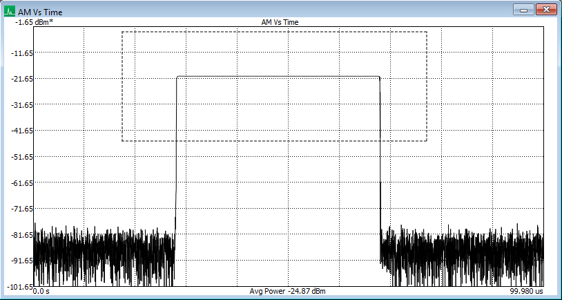
Left click dragging a new zoom region in the plot.
- Click and drag to the left of the y-axis or below the x-axis to pan the reference level or time.
- Hover and scroll to the left of the y-axis or below the x-axis to contract/expand the axis.
- Context menu > Set Axes to manually define axis ranges.
When axes have been modified, an asterisk appears next to the plot unit. Use the context menu to revert to a previous or default scale.
Markers
Left-click within the plot border to place the marker on the closest point. Use left/right arrow keys to move one index at a time. On plots with multiple lines, use up/down arrow keys to jump between them. Activate the delta marker from the context menu to place a reference at the current marker position; select again to disable.
Right Click Context Menu
- Previous Zoom – Restores the previous zoom/scale level; shows how many user zoom levels are active.
- Auto Zoom – Restores the default scale.
- Enable Zoom / Disable Drag Marker – Toggles between zoom drag and marker drag modes.
- Set Axes – Manually define x and y axis ranges.
- Peak Search / Minimum Search – Move the marker to the largest or smallest y-value (enables the marker if disabled).
- Place Delta Marker – Place the reference marker at the current marker position.
- Disable Marker – Disable the marker and delta marker.
- Export – Export all graphs in the plot to a CSV file.
- Save as Image – Save the current plot as an image.
Spectrogram
The spectrogram (waterfall display) shows multiple sweeps over time. Available in sweep, real-time, and interference hunting modes.
Each horizontal line represents one sweep. The x-axis is frequency, the y-axis is time, and amplitude is shown using a color-coded scheme. Enable from the toolbar; resize by dragging the splitter bar below the display.
Left-click to place a marker showing frequency, amplitude, and time. Right-click for the context menu:
- Preferences – Opens spectrogram preferences.
- Clear Spectrogram – Clears the current display.
- Delta Marker – Sets the delta marker at the current position.
- Auto Scale – Sets min/max color scale to the min/max of the currently displayed data.
Preferences:
- Sweep Depth – Number of spectrums stored. When full, the oldest is removed for each new one. Current count and depth are shown in the upper left.
- Time Density – Minimum time each stored spectrum represents. At faster sweep rates, multiple sweeps are accumulated into one stored spectrum.
- Mouse Wheel Scroll Pixels – Scrolling speed when using the mouse wheel.
- Auto Scrolling – When disabled, the display does not advance while viewing past events. Note: once the maximum sweep count is reached, the display scrolls regardless.
- Marker Active – Enables or disables the marker.
- Color Scale – Switch between color spectrum and grayscale gradient.
- Scale to Ref – When enabled, the reference level and bottom of the graticule define the color gradient min/max. When disabled, Min Color and Max Color settings are used.
- Min Color / Max Color (dBm) – Override the amplitude range mapped onto the color gradient when Scale to Ref is disabled.
Persistence
The persistence display shows spectral density over time using color to represent how often a signal appears. Rarely occurring signals appear in light blue; persistent signals progress from blue to green to red.
Two types are available:
- Standard spectrum analysis – Accumulation of the most recent sweeps.
- Real-time mode – Accumulation of approximately 2/3 of a second of spectrum data (1,600–400,000 FFTs per update, depending on RBW).
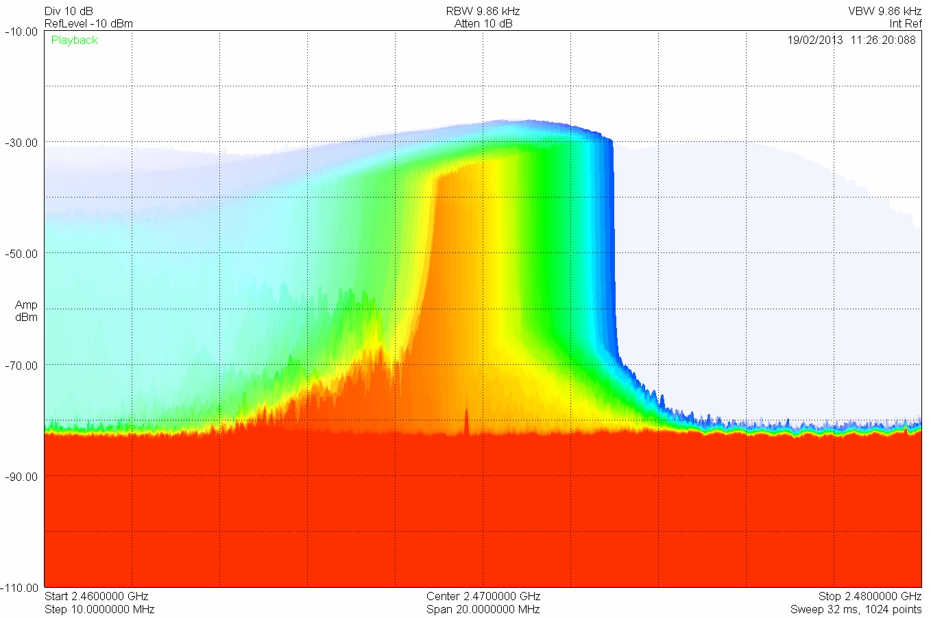
Sweep mode persistence showing the signal from a poorly sheilded commercial microwave oven.
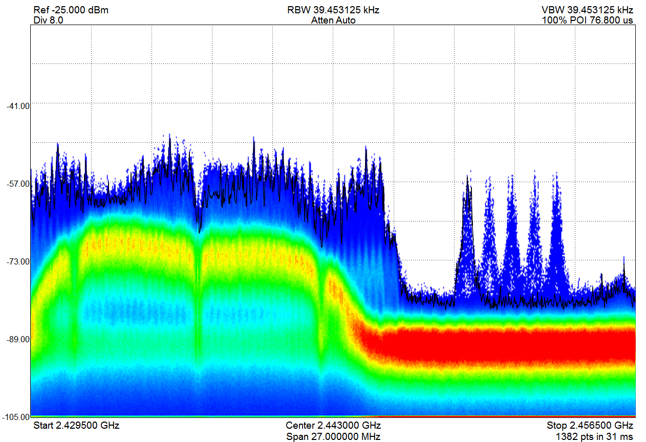
Real-time persistence of a wireless router and Bluetooth headset coexisting in the 2.4GHz ISM band.
SCPI
Spike is programmable via SCPI commands over a TCP/IP socket (default port 5025). The connection and port number can be configured in the preferences menu.
When a SCPI connection is active and a command is received, Spike enters remote operation mode and displays a modal dialog. Press Return to Local or close the dialog to return to local control. See the Spike SCPI programming manual in the SDK download for full programming information.
SCPI Log
When logging is enabled, all received SCPI commands and sent responses are logged with timestamps. Access the log via Utilities > SCPI Log.
- Running counters in the upper left show commands received, responses sent, and total messages.
- Log state (enabled/disabled) is shown in the upper right and toggled in SCPI preferences. Disabling logging saves a few milliseconds of overhead.
- Export – Export the log as a plain text file.
- Clear – Clear the log.
Printing
Use File > Print to print the current graticule view. Use the print preview option to verify the output. Press Single to stop trace updates before printing to guarantee the desired signal is captured.
Saving Images
Use File > Save to Image to save the current graticule view as a PNG, JPG, or BMP. The image resolution matches the graticule resolution at the time of save. For highest resolution, maximize the application and minimize the control panel footprint.
Correction Data
Use File > Manage Correction Data to manage locally cached correction data pulled from Signal Hound devices.
- View Correction Data – Opens the directory containing cached correction data files in Windows Explorer.
- Clear Correction Data – Removes all cached correction data. The device will re-cache its correction file on the next connection.
Use these functions only after device recalibration or if directed by Signal Hound Support. For older SA series devices, back up calibration data before clearing.
Network Devices
Applies to SM200C, SM435C, and PCR4200 devices.
Connecting Networked Devices
Use File > Manage Ethernet Devices to register networked devices by IP address and port. Once registered, the device appears in File > Connect. Default IP and port values are used for new devices. The host IP should be set to the actual NIC address rather than 0.0.0.0 (any).
- Add Device – Adds a new Ethernet device with default settings.
- Delete Device – Removes the selected Ethernet device from the list.
Networked Device Configuration
Used to modify the IP address and port of a networked device. SM200C and SM435C can be configured over USB or UDP; PCR4200 can only be configured via USB.
Access the configuration dialog with no device connected in Spike, then select Utilities > SM Network Configuration or Utilities > PCR Network Configuration.
Configuring Over USB
Connect the device via the provided USB cable. In the Via USB tab, press List Devices to show all networked devices connected via USB. Specify the target device serial number and new network settings, then press Program Device. When Non-Volatile is unchecked, settings do not persist through a power cycle.
Configuring Over UDP
Settings are broadcast in a UDP packet — only one SM200C/435C should be connected to the local network interface at a time. Specify the host address directly rather than using 0.0.0.0 when possible. A failure report when changing subnets may still indicate a successful update.
Path Loss, Limit Line, and Antenna Factor Format
All correction and limit tables are loaded as CSV files (values separated by commas, logical sets separated by newlines). Values are linearly interpolated.
- Path loss tables – [Frequency (MHz), Gain (dB)] pairs describing system component response. Applied at each frequency point. First and last values are extended to the sweep start/stop frequencies — prefix and postfix with zeros to avoid extending corrections beyond the defined range.
- Antenna factor tables – [Frequency (MHz), Antenna Factor (dB/m)] pairs describing antenna response. Same structure as path loss tables; changes measurement units to electric field strength (used in compliance testing).
- Limit lines – [Frequency (MHz), Limit (dBm)] pairs. Tested only within the frequency range of the lowest and highest defined points.
Managing Path Loss Tables
The path loss table dialog manages up to 7 path loss tables and one antenna factor correction table. Table file names are stored in presets and loaded automatically; if a file has been moved or renamed, the table is removed on preset load.
Path loss is applied in two ways:
| Method | Description |
| Full | Applied at each output frequency point in the measurement. |
| Single | Applied at a single frequency (usually center frequency) — equivalent to a flat dB offset. |
Path loss application by mode:
| Measurement Mode | Path Loss Method |
| Swept spectrum analysis | Full |
| Real-time spectrum analysis | Single |
| Zero-span | Single |
| Harmonics viewer | Full |
| Scalar network analysis | Full |
| Phase noise | None |
| Modulation analysis | Single |
| EMC precompliance | Sweeps: Full, QP Detector: Single |
| Analog demodulation | Single |
| Interference hunting | Full |
| Measuring receiver | None |
| Spectrum Emission Mask | Full |
Managing Limit Lines
The limit line dialog configures up to 6 limit lines, each stored as frequency/amplitude pairs with interpolated test points. Limit lines can be loaded from CSV files and are stored in presets.
- Enabled – Activates or deactivates the limit line.
- Name – Displayed on the plot if Show Result is checked.
- Trace – Sets the trace the limit line acts upon.
- Type – Sets whether the line is an upper or lower bound.
- Reference – Sets whether frequencies are fixed or relative (to center frequency).
- Convert To – Converts the reference mode between fixed and relative, recalculating points based on current screen position.
- Interpolation – Linear or logarithmic interpolation between points.
- Color – Color of the limit line.
- Pause On Break – When enabled, Spike switches to single step mode if the limit is violated.
- Show Line / Show Result – Controls visibility of the line and pass/fail status on the plot.
- Offset – dB offset applied to all points in the line.
- Points To Build – Number of points to use when building a line from the current trace.
- Build Line – Constructs new limit line data from the current trace.
- Modify Points – Opens the limit line table editor for editing individual points.
- Copy To – Copies points, type, reference, and offset to a selected limit line.
- Number of Points – Displays the current point count.
Audio Player
Access via Utilities > Audio Player. Plays broadcast audio demodulated from the input signal. Set the center frequency via the arrow keys, fine-tune buttons, or manual entry. Bandwidth and demodulation type are also configurable, along with audio low-pass and high-pass filter cutoff frequencies. All audio settings except center frequency are saved with presets.
Frequency Difference Meter
Determines the frequency difference between two stable oscillators, displayed as a digital readout and a zero-centered meter. Scale options: 10⁶, 10⁷, 10⁸, 10⁹, 10¹⁰, 10¹¹ parts.
Connect an external reference to the BNC port and activate it via the file menu (if no external reference is present, the internal timebase is used). Connect the oscillator to be measured to the RF input port. Set the reference level ~5 dB above the input signal. Observe the frequency offset (Measured − Desired) and adjust the scale radio buttons as the frequency difference narrows. Allow several seconds for the meter to settle on the smallest scale settings.
Adjusting Your Timebase
Access via Utilities > Timebase Adjustment. Adjusts the Signal Hound's internal 10 MHz oscillator against a high-precision external CW source connected to the RF input port. The correction is stored per device serial number on the local PC and applied in all future sessions for that device on that PC.
Steps:
- Connect the high-precision source to the RF input port.
- Disconnect any cables from the reference in/out BNC port.
- Set the reference level ~5 dB above the expected signal.
- Set the input frequency to match the oscillator frequency.
- Verify the frequency offset reading is stable.
- Press Adjust Timebase.
Press Restore Default at any time to revert to factory calibration settings (no input signal required).
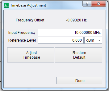
Timebase adjustment utility.
Spur Rejection
When enabled, additional signal processing attempts to remove spurious mixing products. Roughly doubles sweep time. Effective for steady signals; should not be used for pulsed RF or modulated signals. Not available in real-time mode.
Networked Speed Test
Tests the throughput of a connected networked device (SM200C, SM435C), displayed in Gbps updated each second. Uses UDP jumbo packets. For SM200C/SM435C, sustained speed should exceed 8 Gbps.
GPS Control Panel
Access via Utilities > GPS Control Panel. Spike can use a GPS device for timestamps and coordinates in sweep recording, mapping, LTE measurements, and more. GPS can be internal (SP145, SM200, SM435) or external (serial/USB). GPS data updates approximately once per second. Current lock status is shown in the control panel and the status bar.
For internal GPS, the Platform Model can be set to Stationary or Portable. Use Portable for any mobile scenario to maintain lock when velocity is non-zero.
Windows: Select the COM device from the dropdown. Press Refresh COM Devices if a GPS was connected after opening the panel.
Linux: Enter the serial device name (e.g., ttyACM0) under Device Name. Use ls /dev | grep tty to find the device name.
Press Connect to establish communication. The panel warns if the device cannot be detected or if the NMEA data does not contain a valid RMC sentence.
Status messages:
- Comm Error – No valid RMC string found. Likely an incorrect baud rate — verify in Device Manager.
- Locked/Unlocked – Echoes the RMC lock status. Coordinates are not used while unlocked.
- Unable to Connect GPS – Verify COM port and baud rate, and ensure the device is properly configured.
GPS Disciplined Timebase
(SM series spectrum analyzers only)
The SM uses its internal GPS to discipline the internal timebase and clocks, improving frequency measurement accuracy and timestamping. Discipline is enabled by default — connect the supplied antenna to begin.
GPS states shown in the Spike status bar:
- GPS Unlocked – Antenna disconnected or not yet locked. Allow several minutes after connecting.
- GPS Holdover – GPS unlocked; using the last stored holdover value (e.g., "GPS Holdover (3d19h)").
- GPS Locked – Lock achieved; discipline has not yet started. Lock must be held for several minutes before discipline occurs.
- GPS Disciplined – SM has been disciplined to the GPS and continues to discipline periodically.
The last known timebase correction is stored at C:\ProgramData\SignalHound\cal_files\sm########gps.bin. Deleting this file reverts to the factory calibration. The newest correction value (timestamped) is always used.
BB60D GPIO Controls
Access via Utilities > BB60D UART Controls.
- UART Rate – Select the UART clock rate from predefined values.
- Imm Config/Write – Directly transmit up to 8 bits over the UART port immediately.
- UART Sweep – Transmit up to 8 UART bytes at specific sweep frequencies. Useful for intra-sweep antenna switching or controlling external devices. A byte is transmitted when the sweep frequency crosses each user-defined frequency. When enabled, overrides the 10 MHz reference output.
SP145 GPIO Controls
SM GPIO Controls
Access via Utilities > SM GPIO Controls. Controls the 8 GPIO pins on the DB15 port of SM200 and SM435 spectrum analyzers in two modes:
- Fixed Output Mode – Sets GPIO pins to fixed values. Device measurements stop while updating pin states. The GPIO remains fixed until disabled or modified.
- Sweep Output Mode – Configures a sequence of frequency/GPIO value pairs. When the sweep crosses a specified frequency, the GPIO pins are updated to the associated values. The first frequency should be 0 Hz to set initial pin states. Up to 8 frequency/GPIO steps can be configured. Frequency resolution is 40 MHz in standard sweep mode and 160 MHz in real-time swept mode.
Demo Mode
If Spike is opened with no device connected, a dialog offers the option to launch a demo device with simulated signals. Available demo modes: Sweep, Zero-Span, Digital Demodulation, Interference Hunting, Spectrum Emission Mask, Harmonics, and Mapping.
Managing Licenses
The License Manager dialog (accessed from the Utilities menu) adds, activates, removes, and displays details about locally stored licenses. Active licenses are listed on the left with associated serial numbers; expired licenses appear in red. Clicking a license shows its details and enables actions on the right.
Adding and Activating a License
An internet connection is required for activation. After activation, the license is stored locally and no internet connection is needed for subsequent use.
- Ensure Spike is up to date.
- Navigate to your account page on the Signal Hound website and click Licenses in the sidebar.
- Click Copy to copy your license key to the clipboard.
- In Spike, open the License Manager from the Utilities menu.
- Click Add License, paste the license key into the text field, and click OK.
- When prompted, enter the serial number of the Signal Hound spectrum analyzer to associate with the license. The license becomes active once associated with a serial number.
Removing a License
Select the license from the list and press Remove License. This removes the license from the local machine only — the license itself is unaffected and can be re-added on this or another machine.
Refreshing a License
If a license was renewed or otherwise altered, press Refresh License to update the locally stored information.
Troubleshooting
"Device Not Found" (All Devices)
- Ensure the device is plugged in and the LED is solid green. If not, unplug and reconnect the device, then use File > Connect.
- If the LED is solid green but the device still won't connect, see the device-specific tips below.
LED is solid green but device won't connect:
- Early BB60A units may require a power cycle after the PC restarts or wakes from hibernation.
- If it is the first time the device has been connected, the PC may take several seconds to install drivers. Wait until the device appears with its Signal Hound name in Device Manager.
- If a power cycle doesn't resolve the issue, the drivers may not have installed correctly. See Driver Installation.
Device connected but no solid green LED:
- BB series: Power cycle by disconnecting the USB from the analyzer end. For Y-cable devices, ensure both USB ends are connected to the PC before reconnecting to the device. Try a different USB port; avoid charging-only ports. Update power management settings.
- SA series: Disable anti-virus software. In Device Manager under Universal Serial Bus Controllers, find Serial Converter A/B, open Properties > Advanced, and ensure Load VCP is unchecked.
"Device Not Found" (BB60, SM200A/B, SM435B)
Ensure the LED is solid green and that drivers are installed — check Device Manager under Universal Serial Bus Controllers for the Signal Hound device while it is connected.
If the LED is not solid green: update USB 3.0 drivers via Windows Update and the PC manufacturer's website. Unplug the device before updating drivers, restart afterwards, and verify operation.
"Device Not Found" (SA44, SA124)
- Ensure cables are properly secured and the LED is solid green.
- Install the USB drivers from the Spike download page.
- In Device Manager, find Serial Converter A/B under Universal Serial Bus Controllers, open Properties > Advanced, and ensure Load VCP is unchecked.
- Enable High Performance power plan in Control Panel > Power Options to ensure adequate USB power.
- Disable anti-virus software.
Device Disconnects During Operation
- Disable anti-virus software.
- Update power management settings.
- Update USB drivers (see BB60/SM200A/B/SM435B section above).
The Device is Not Valid
Power cycle the device and restart the PC. If the issue persists, contact Signal Hound.
"IF Overload" on Program Startup
Normal behavior for a short time (<1 second) after launching the software or connecting the device. Part of the hardware startup process.
Power Management Settings
Perform this step with the device disconnected. Set the power plan to **High Performance** in **Control Panel > Power Options** (may require clicking Show Additional Plans). Also consider disabling Selective Suspend in USB Settings under Advanced Power Options.
Error Code 48: Software for This Device Has Been Blocked (BB60C)
Drivers were improperly installed. To resolve:
- Connect the BB60C and open Device Manager.
- Under Universal Serial Bus Controllers, find the BB60C, right-click, and uninstall the driver (select any option to also delete driver files).
- Disconnect the BB60C.
- Navigate to C:\Program Files\Signal Hound\Spike\drivers\x64 (or x86 for 32-bit Windows).
- Right-click cyusb3.inf and select Install.
- Reconnect the BB60C and launch Spike.
Device Does Not Work in a Windows Virtual Machine (BB60C Only)
Signal Hound devices are not officially supported in virtual machines, but some configurations have worked:
- Use the latest version of VMware on a PC with USB 3.0 and a 4th-generation or later Intel i5/i7 CPU.
- Ensure USB 3.0 SuperSpeed is enabled for the virtual machine (often disabled by default).
- Manually install the BB60C drivers if the Spike installer fails to do so. See Driver Installation.
Calibration and Adjustment
Contact Signal Hound for information regarding calibration software and required equipment.
Appendix
Using Multiple USB 3.0 Devices on Linux
The default USB memory allocation on Linux is 16 MB. A single Signal Hound USB 3.0 device stays within this limit, but two devices will exceed it and may cause connection issues or crashes. Increase the allocation with:
sudo sh -c 'echo 32 > /sys/module/usbcore/parameters/usbfs_memory_mb'
Use N × 16 MB where N is the number of simultaneous devices. A system restart may be required.
Command Line Options
- --hidden – Hides the user interface including the taskbar entry. For headless SCPI operation. The following dialogs are suppressed: No device connected, Multiple devices connected, Connecting device, SCPI remote operation notification. Close the application via SCPI commands or Task Manager.
- --preset=n – Load quick preset number n (1–9) after launching. Requires one connected device that auto-connects and a preset created with that device type.
- --preset-user="filename.ini" – Load a user preset on startup. Specify the full file path (use quotes if the path contains spaces). Requires exactly one connected device and a preset created with that device type.
- --scpi-port=n – Set the SCPI port after launch (integer ≤ 65535). Useful for running multiple Spike instances with different SCPI ports.
MATLAB® Runtime Installation Instructions
LTE measurements require the MATLAB® runtime (and on Windows, the VS2019 C++ redistributable libraries).
Installing the MATLAB Runtime
Download R2021b (9.11) from www.mathworks.com/products/compiler/matlab-runtime.html.
- Windows: Run the 64-bit installer and install to the default folder. If the installer cannot add the runtime to the system PATH (often due to the PATH variable exceeding 2047 characters), manually add C:\Program Files\MATLAB\MATLAB Runtime\v911\runtime\win64 to the system PATH via the registry editor or environment variable editor. A PC restart is required before Spike detects the runtime.
- Linux: Run sudo -H ./install and install to the default folder (/usr/local).
Windows Only: VS2019 C++ Redistributable Library
Download and install the 64-bit (non-ARM) libraries from the Microsoft Visual C++ redistributable downloads page.
Load Times
The MATLAB runtime initializes the first time LTE measurements are accessed each session, typically taking 3–15 seconds. Anti-virus software can significantly increase this time — consider disabling real-time AV monitoring to reduce load times.
Constellation Mappings
For all non-differential PSK/QAM modulations, the mappings can be observed directly in the custom modulation editor by loading a default constellation and inspecting the table.
For other modulations, see below.
DBPSK
| Data | Phase Change |
| 0 | 0° |
| 1 | 180° |
DQPSK
| Data | Phase Change |
| 0 | 0 |
| 1 | +π/2 |
| 2 | −π/2 |
| 3 | π |
π/4 DQPSK
| Data | Phase Change |
| 0 | +π/4 |
| 1 | +3π/4 |
| 2 | −π/4 |
| 3 | −3π/4 |
D8PSK
| Data | Phase Change |
| 0 | 0 |
| 1 | +π/4 |
| 2 | +3π/4 |
| 3 | +π/2 |
| 4 | −π/4 |
| 5 | −π/2 |
| 6 | π |
| 7 | −3π/4 |
OQPSK
Offset QPSK: same as QPSK, except the Q channel is delayed by ½ symbol.
2-FSK
| Data | Frequency Offset (normalized) |
| 0 | −1 |
| 1 | 1 |
4-FSK
| Data | Frequency Offset (normalized) |
| 0 | −1 |
| 1 | −1/3 |
| 2 | 1 |
| 3 | 1/3 |
8-FSK
| Data | Frequency Offset (normalized) |
| 0 | −1 |
| 1 | −5/7 |
| 3 | -3/7 |
| 2 | -1/7 |
| 6 | 1/7 |
| 7 | 3/7 |
| 5 | 5/7 |
| 4 | 1 |
16-FSK
| Data | Frequency Offset (normalized) |
| 0 | −1 |
| 1 | −13/15 |
| 3 | -11/15 |
| 2 | -9/15 |
| 6 | -7/15 |
| 7 | -5/15 |
| 5 | -3/15 |
| 4 | -1/15 |
| 12 | 1/15 |
| 13 | 3/15 |
| 15 | 5/15 |
| 14 | 7/15 |
| 10 | 9/15 |
| 11 | 11/15 |
| 9 | 13/15 |
| 8 | 1 |
Manual Gain/Atten Settings (BB60)
All settings must be set to non-automatic values to override automatic settings. The preamplifier setting does not affect the measurement itself but must be switched from Auto for manual selections to take effect.
Gain settings:
| Gain | Description |
| 0 | Preamplifier off, add 5 dB to attenuator |
| 1 | Preamplifier off, no additional attenuation |
| 2 | Preamplifier on, add 5 dB attenuation |
| 3 | Preamplifier on, no additional attenuation |
Attenuation settings:
- 0–20 dB: Adds 0 to 20 dB of attenuation plus any contribution from the gain setting.
- 30 dB: Adds 30 dB of attenuation; at this level the effects of Gain 0 and Gain 2 are equivalent to Gain 1 and Gain 3 respectively.
Warranty and Disclaimer
©2013–2026 Signal Hound. All rights reserved.
Reproduction, adaptation, or translation without prior written permission is prohibited, except as allowed under copyright laws. The information in this manual is subject to change without notice. Signal Hound makes no warranty of any kind with regard to this material, including but not limited to the implied warranties of merchantability and fitness for a particular purpose. Signal Hound shall not be liable for errors contained herein or for incidental or consequential damages in connection with the furnishing, performance, or use of this material.
Refer to the End User License Agreement for additional warranty and disclaimer information covering the Spike software.
Credit Notice
Windows® and Excel® are registered trademarks of Microsoft Corporation in the United States and other countries. Intel® and Core™ are trademarks or registered trademarks of Intel Corp. in the United States and other countries. LabVIEW® is a registered trademark of National Instruments Corporation. MATLAB® is a registered trademark of The MathWorks, Inc. The Bluetooth® word mark and logos are registered trademarks owned by Bluetooth SIG, Inc.; use by Signal Hound is under license.
References
- ANSI C63.2 — American National Standard for Electromagnetic Noise and Field Strength Instrumentation, 10 Hz to 40 GHz – Specifications, American National Standards Institute, January 1996.
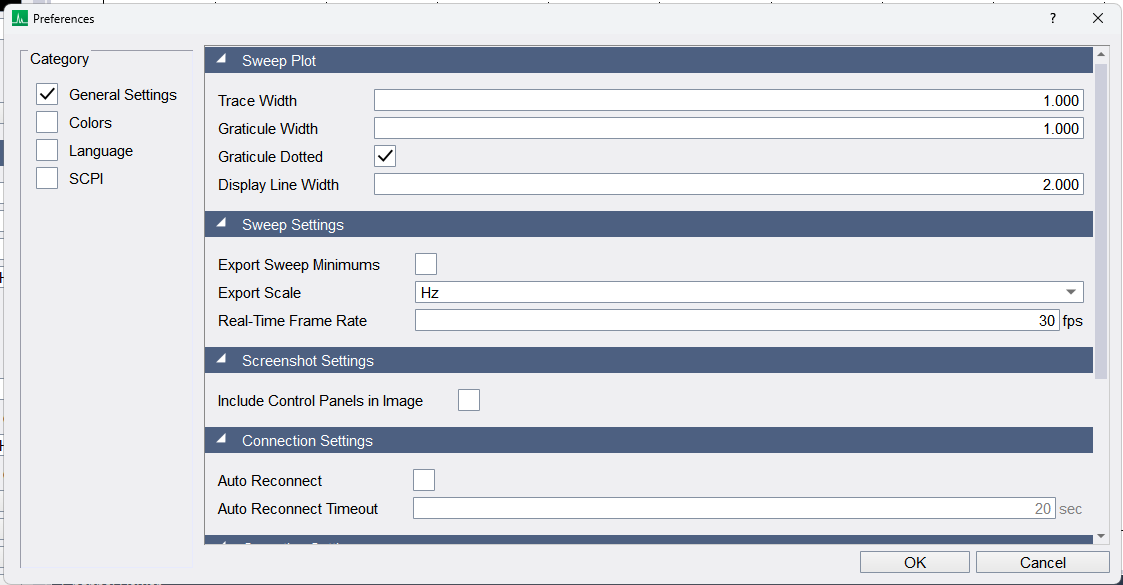

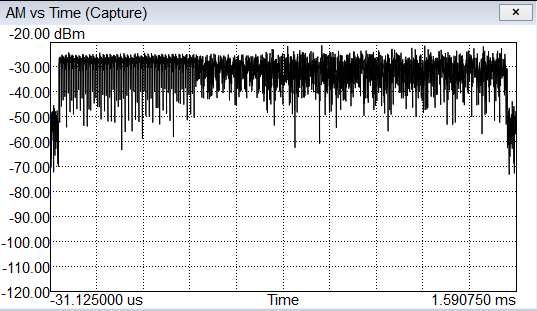
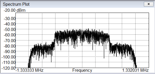
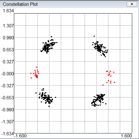
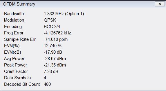
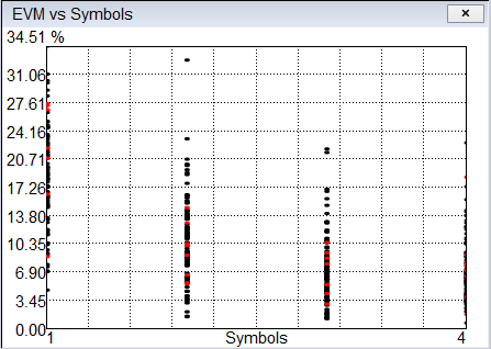
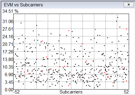
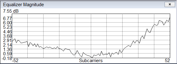
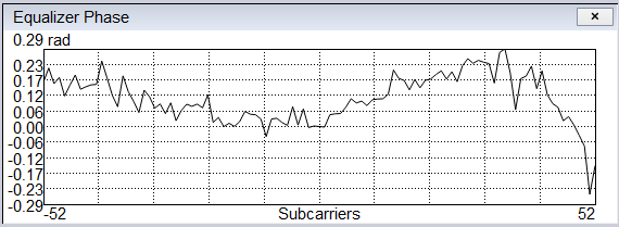
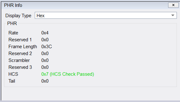
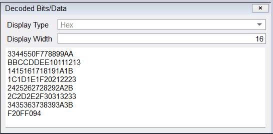
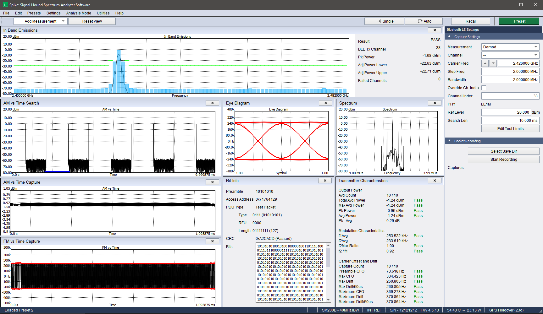
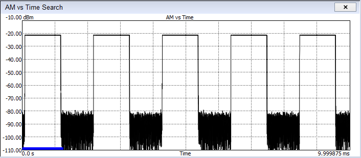
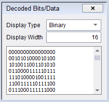
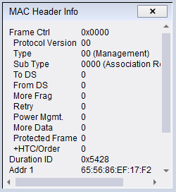

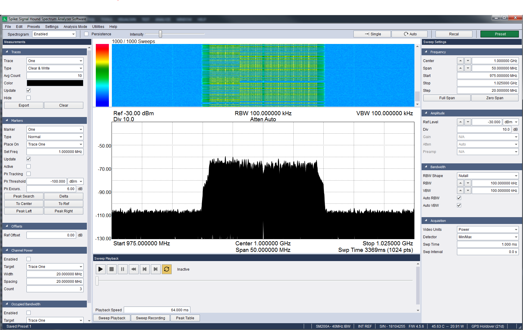
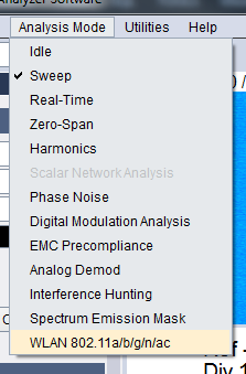
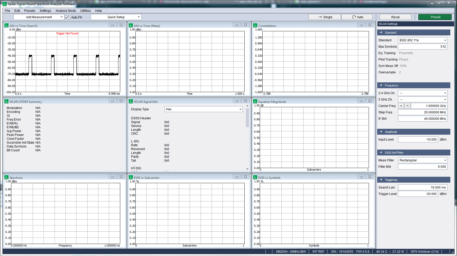
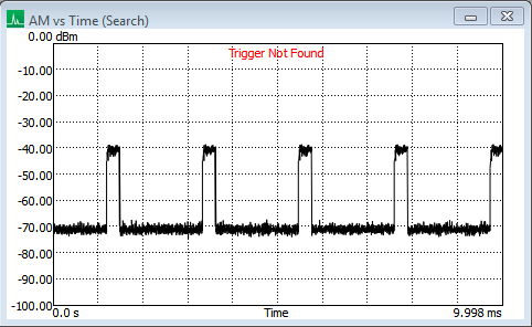
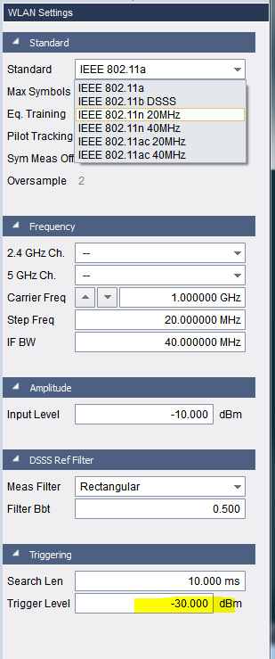
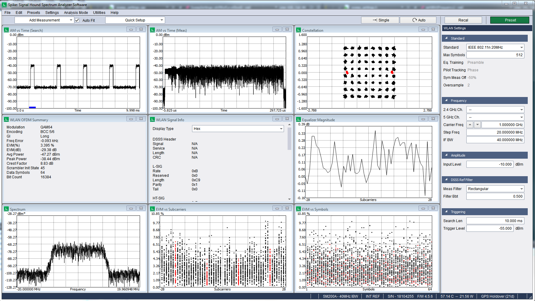

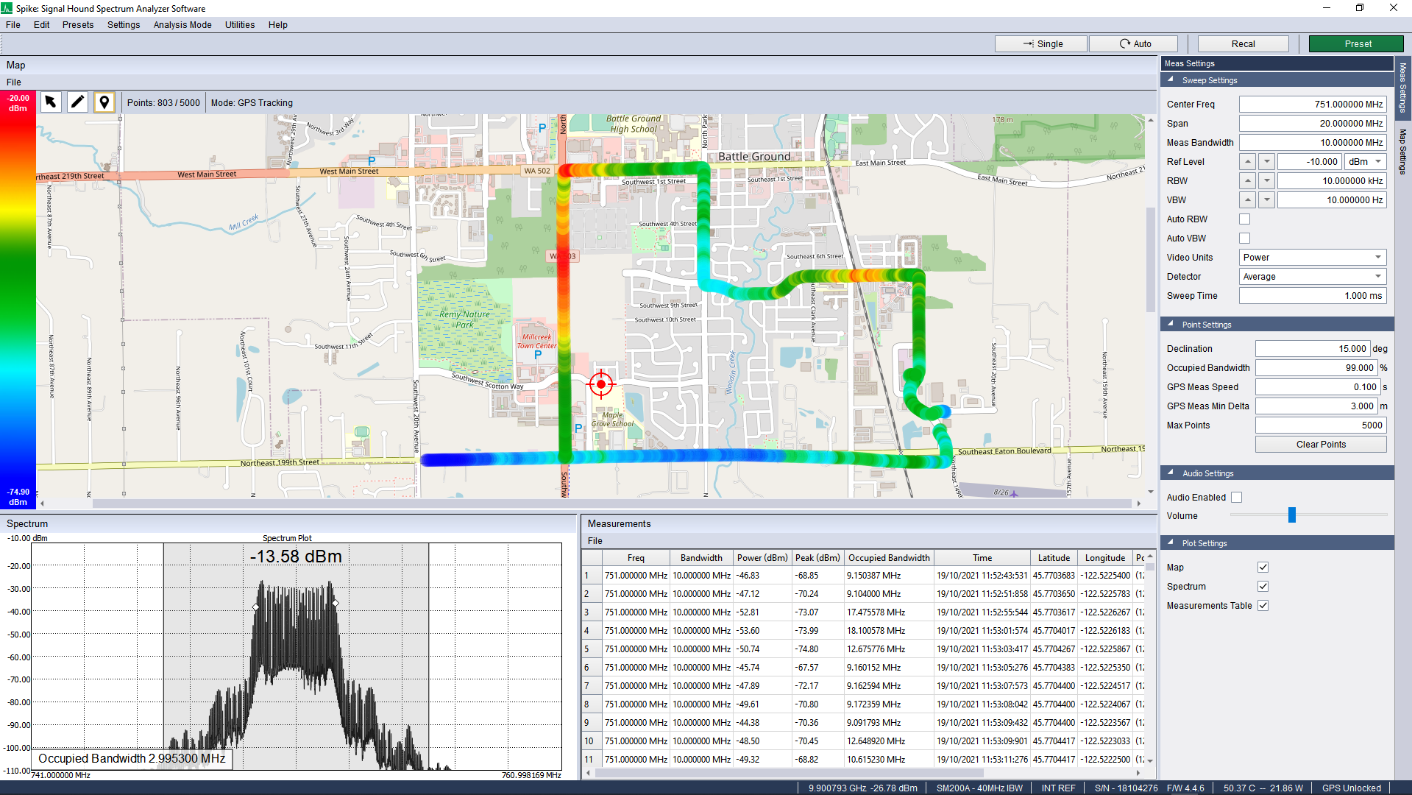
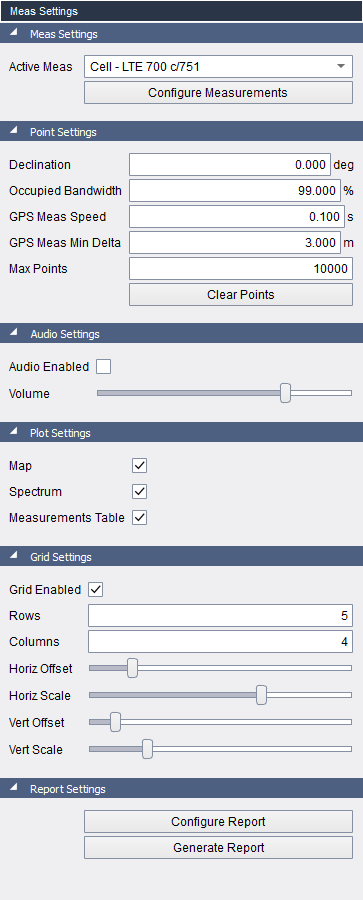
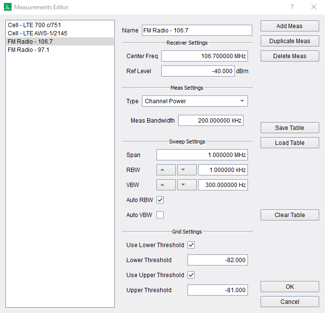
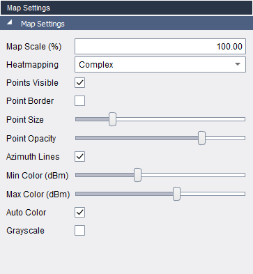
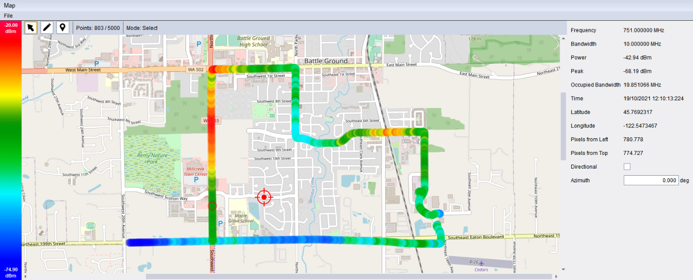
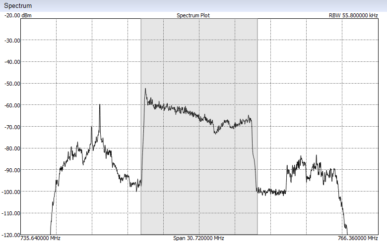
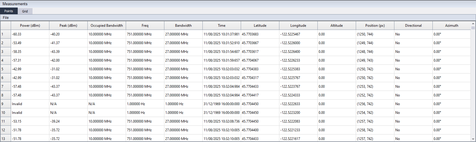
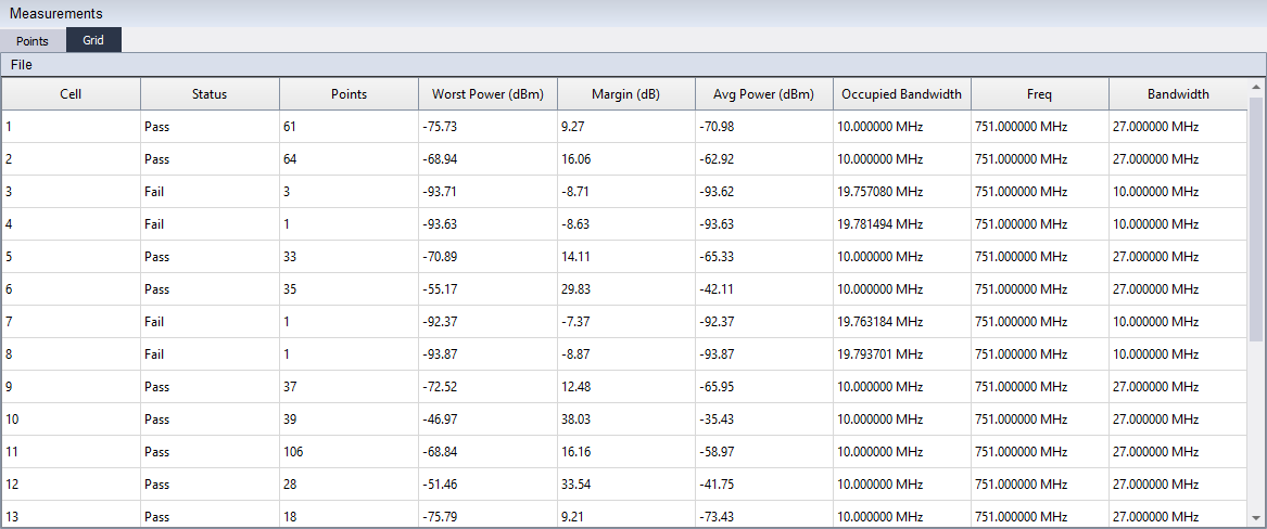
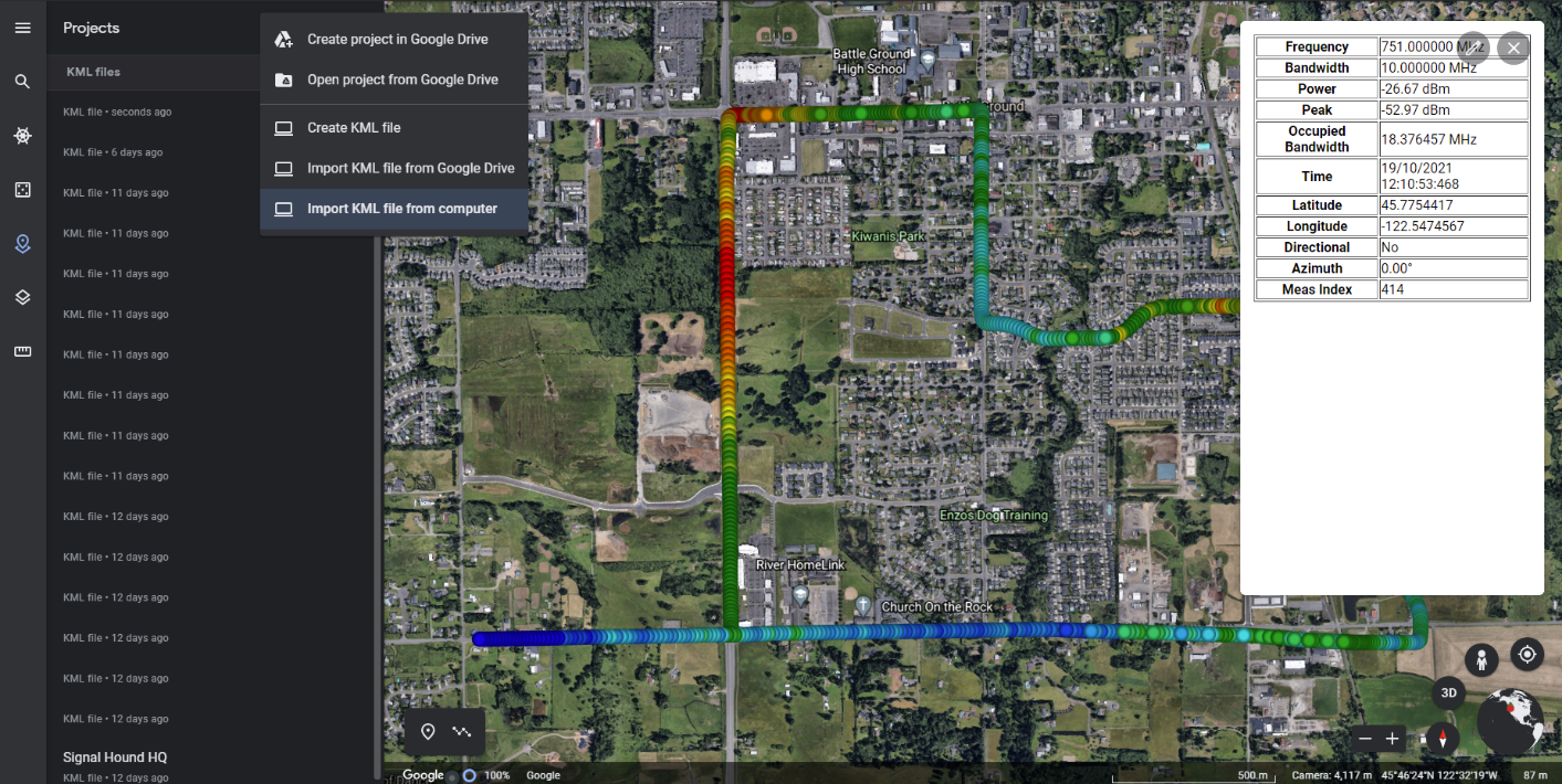
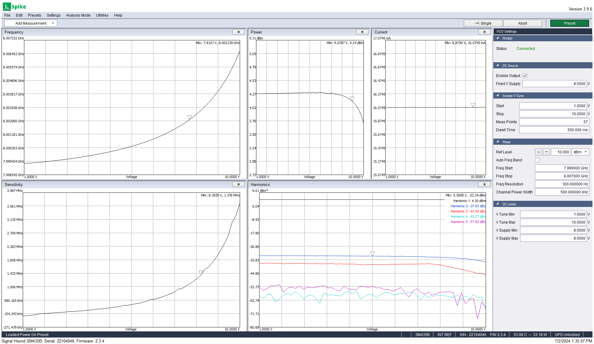
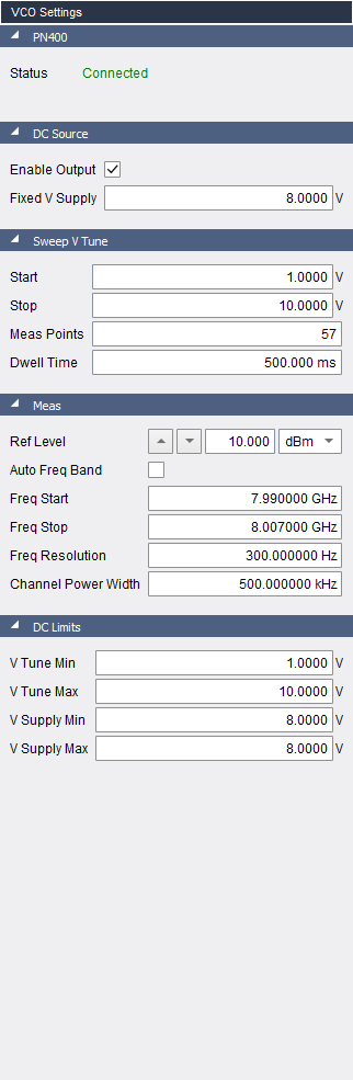
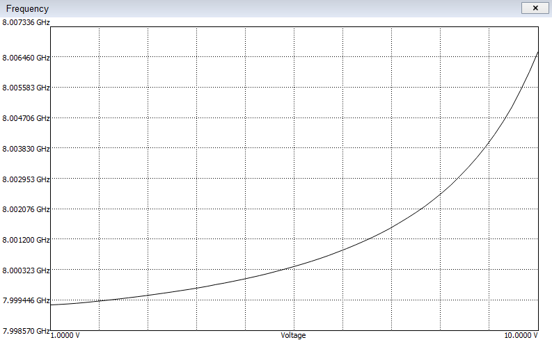
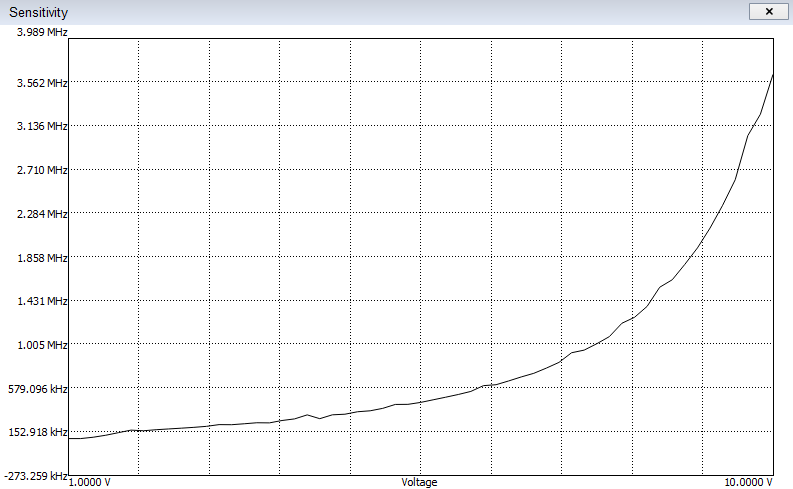
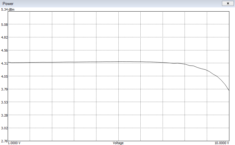
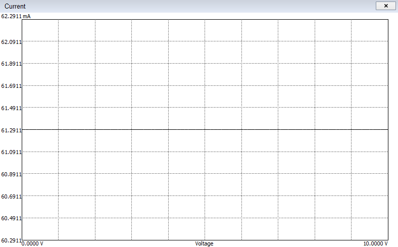
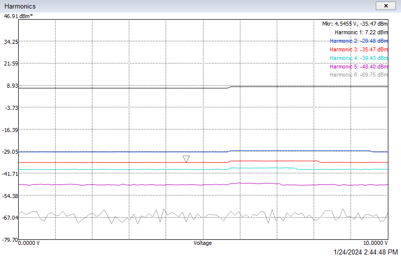
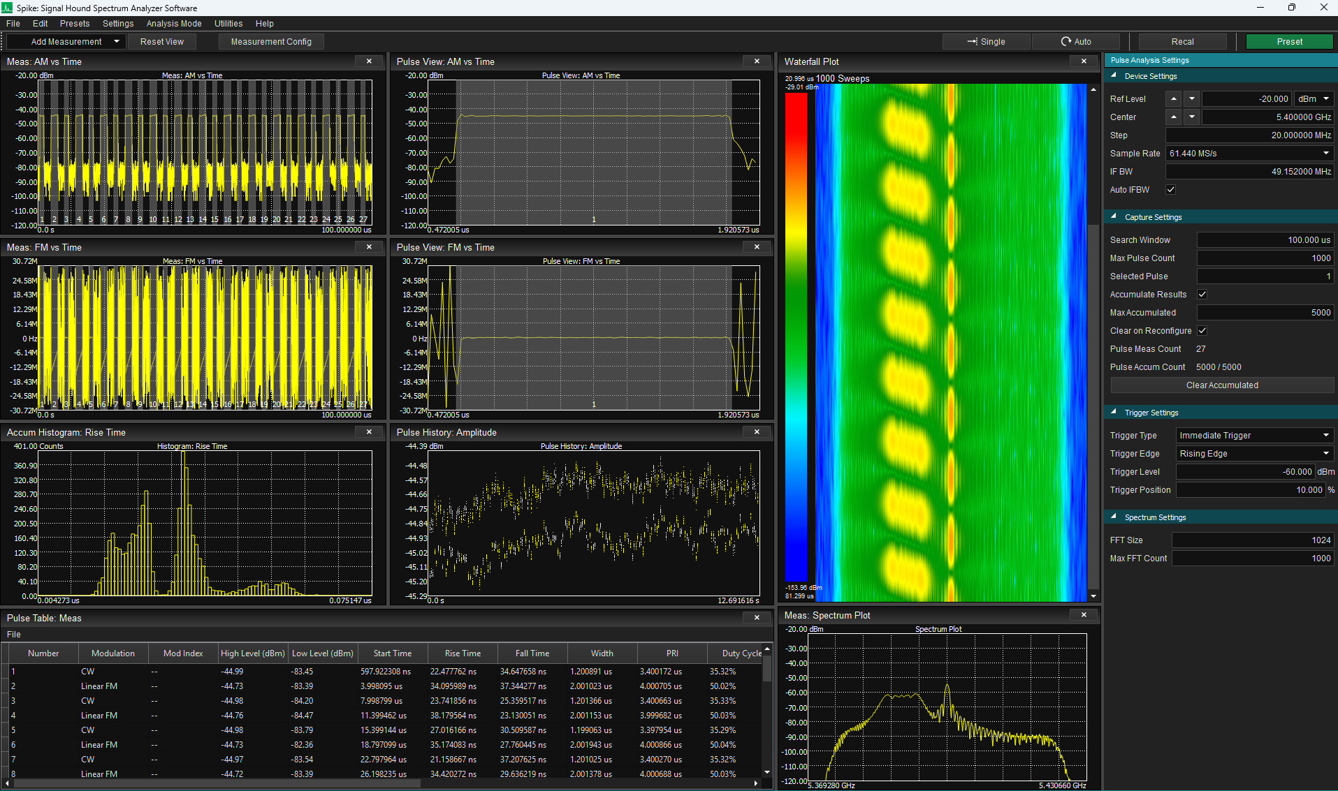
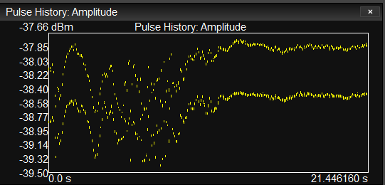
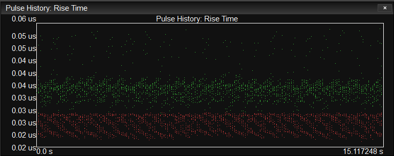
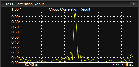
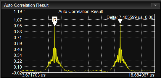
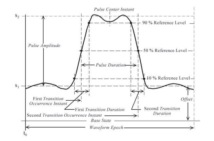
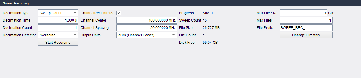
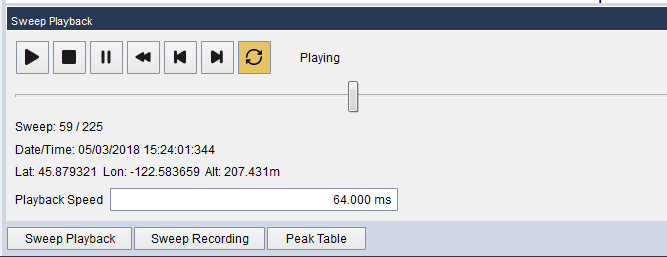
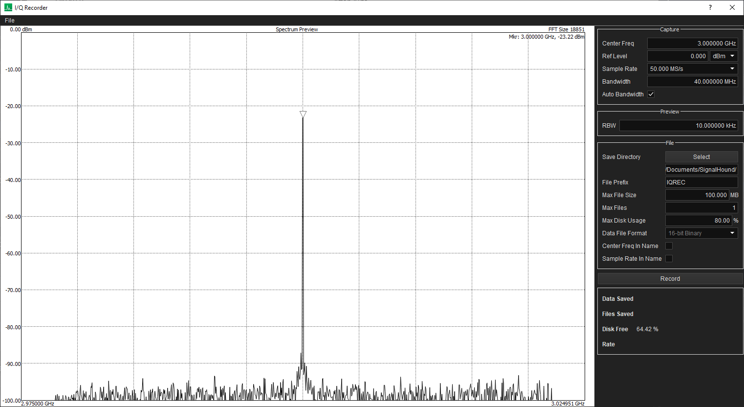

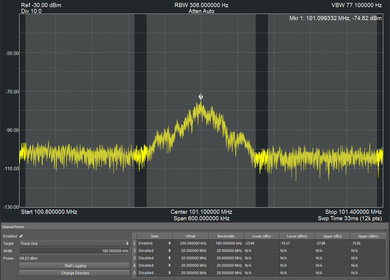

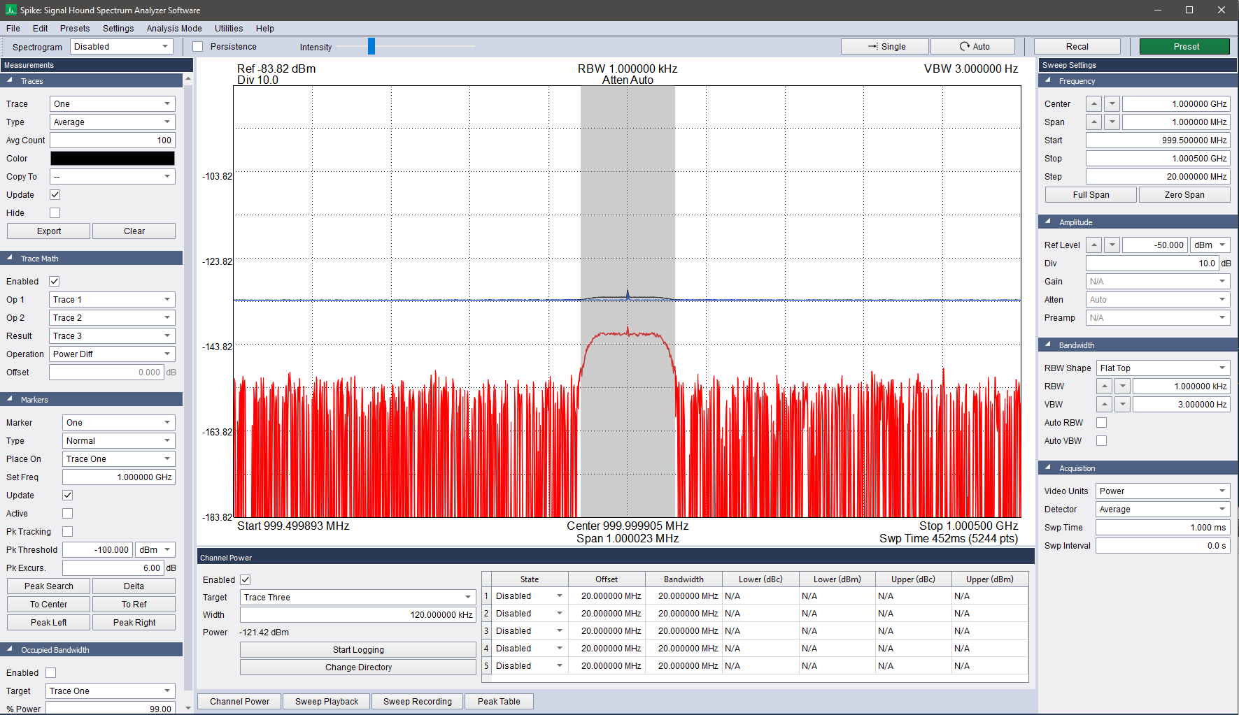
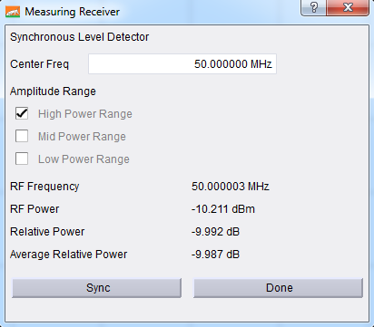
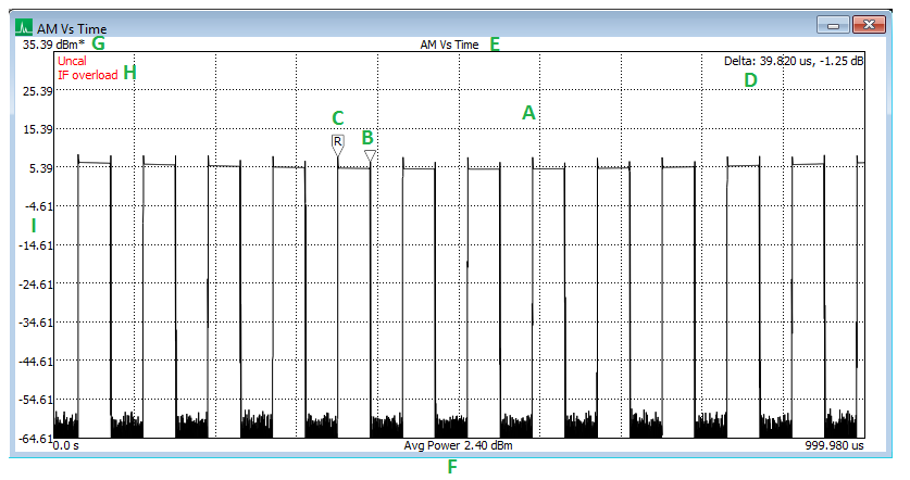
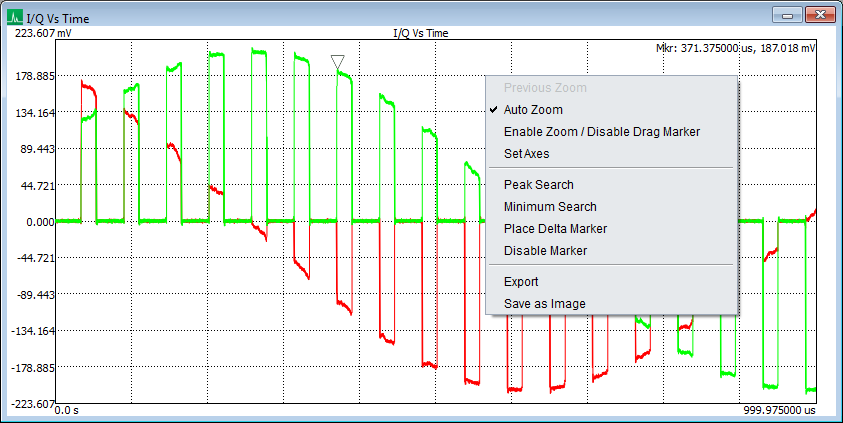
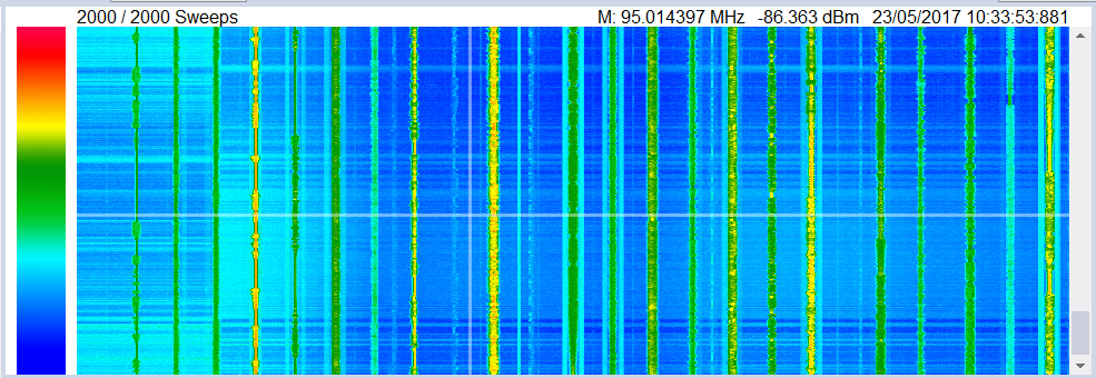
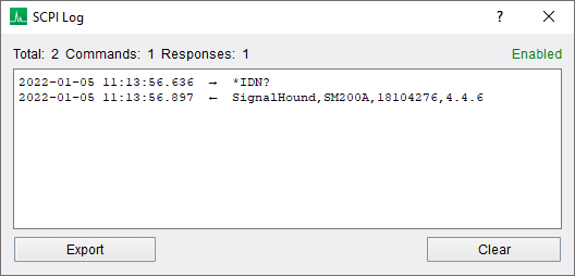
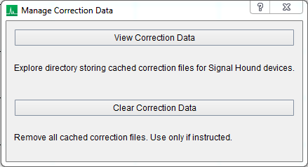
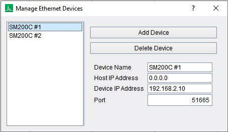
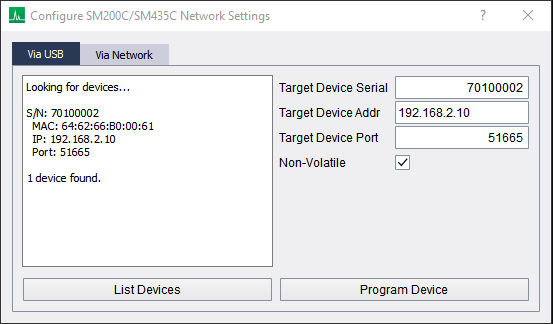
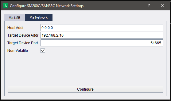
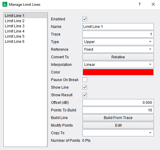
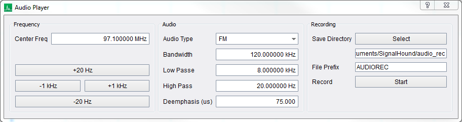
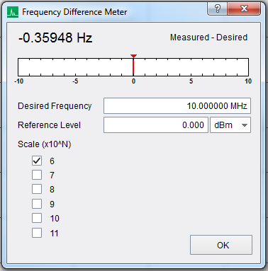
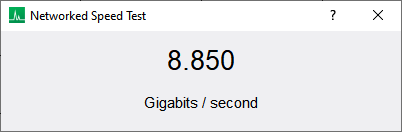
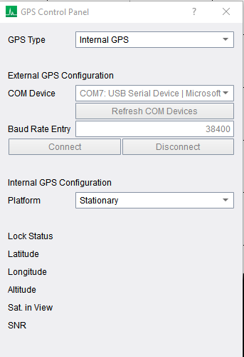

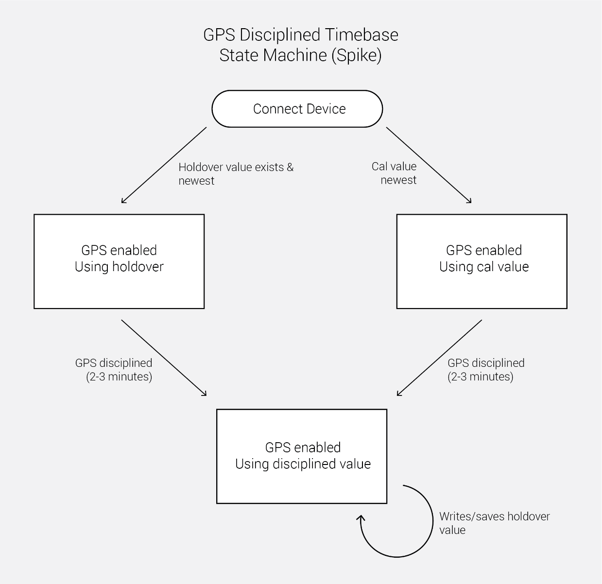
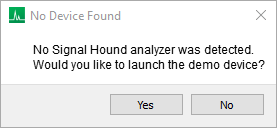
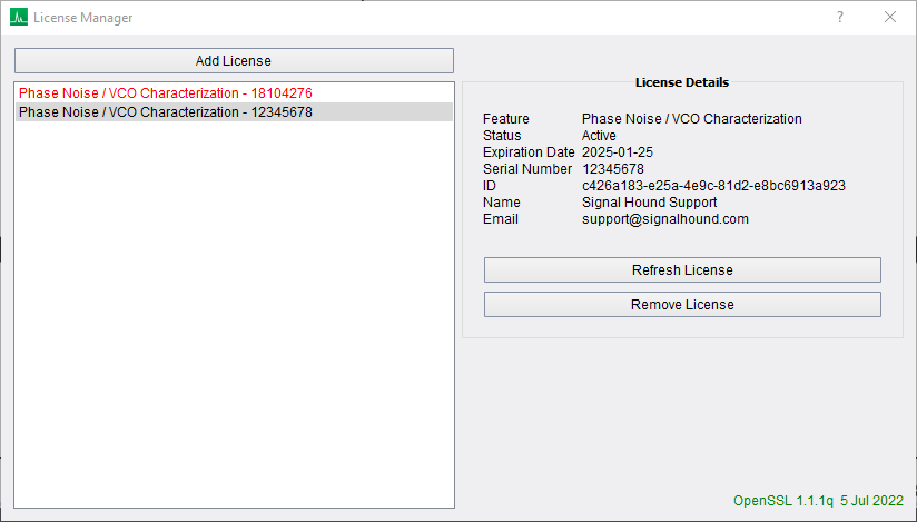

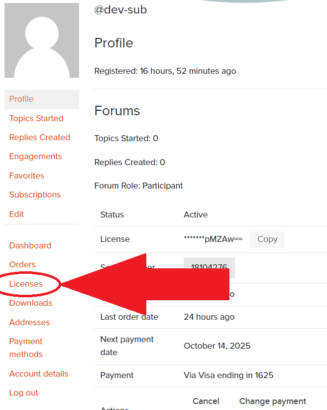
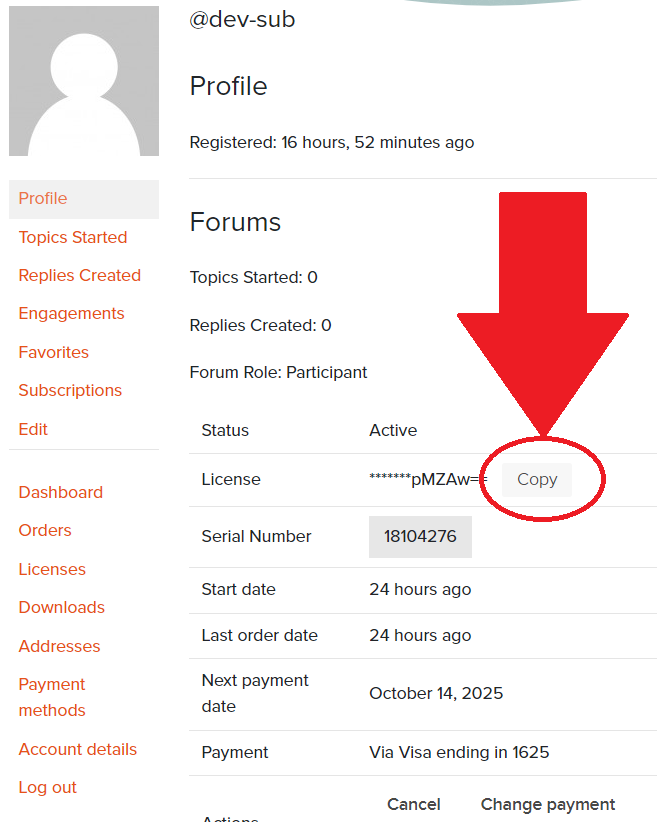
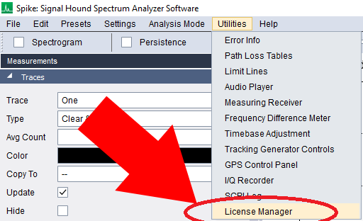
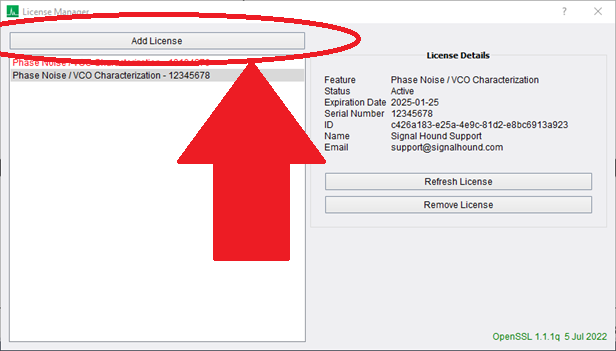
 1.17.0